
Week 1-3: Rule101#
The pattern — Part I
Chapter 0 claims every method this semester is optimize a functional subject to constraints. Here it appears twice:
Functional |
Constraint |
Multiplier / solution |
|---|---|---|
likelihood \(\prod f(x_i-\mu)\) |
the sample mean must be optimal |
the Gaussian (below) |
entropy \(-\int f\ln f\) |
known mean and variance |
the Gaussian again (Chapter 0) |
Two unrelated principles, one curve. The derivation below is the first of them; you do not need Chapter 0 to follow it.
The origin of statistics: why the bell curve?#
Before diving into means and variances, it’s worth asking a more basic question: why does so much of statistics revolve around one particular curve, the Gaussian? The answer has a clean historical and mathematical origin, and walking through it will motivate almost everything else in this section.
A practical problem: combining noisy measurements#
Imagine an early 19th-century astronomer repeatedly measuring the position of a star. Every observation gives a slightly different number,
due to measurement error, yet everyone agrees there is a single true position, \(\mu\). Astronomers and geodesists had long used the arithmetic mean \(\overline{x}\) as their best estimate of \(\mu\), but until the early 1800s, nobody had shown why the mean should be the right choice rather than, say, the median or some other combination of the data.
This is the problem Carl Friedrich Gauss tackled in Theoria Motus (1809), and his solution is what ties the normal distribution directly to an ordinary differential equation.
Setting up the likelihood#
Suppose measurement errors follow some (unknown) probability density \(f(e)\), symmetric about zero. Then, given a candidate true value \(\mu\), the probability (likelihood) of observing the data you actually got is
The best estimate of \(\mu\) is the one that maximizes \(L(\mu)\) — the value that makes the observed data most probable. Taking logs (to turn the product into a sum, which is easier to differentiate) gives the log-likelihood
Differentiating with respect to \(\mu\) and setting the result to zero (the usual condition for a maximum) gives
Note that this condition holds for any error density \(f\) — nothing Gaussian has been assumed yet.
The key constraint: forcing the mean to be optimal#
Gauss then imposed the requirement he was really after: whatever \(f\) turns out to be, the solution to the equation above should always be \(\mu = \overline{x}\), no matter which sample was drawn. This is a strong demand — it is not automatically true for an arbitrary \(f\), and it is exactly the extra assumption needed to pin down the shape of \(f\).
It turns out this holds for every possible sample only if \(\varphi\) is a straight line through the origin,
Why linearity is required
If \(\varphi(e) = -he\), then
Setting this to zero gives \(\mu = \overline{x}\) automatically, for any sample. Try any nonlinear \(\varphi\) and this stops being true in general — linearity is what makes the mean universally optimal.
Why is linearity the only option?
Since everything here is shift-invariant, set \(\overline{x}=0\) without loss of generality. The requirement becomes: for any deviations \(e_1,\dots,e_N\) with \(\sum_i e_i = 0\), we need \(\sum_i \varphi(e_i) = 0\).
\(N=2\) forces \(\varphi\) to be odd. Take \(e_1=d,\ e_2=-d\):
\(N=3\) forces additivity. Take \(e_1,e_2,e_3=-(e_1+e_2)\):
Using oddness, \(\varphi(-(e_1+e_2)) = -\varphi(e_1+e_2)\), so
This is Cauchy’s functional equation.
Solving Cauchy’s equation. Its solutions are linear, \(\varphi(e)=ke\), provided \(\varphi\) satisfies some mild regularity condition (continuity at a point, monotonicity, or boundedness on an interval) — without such a condition, pathological non-linear solutions exist, but they require the axiom of choice and are nowhere continuous. Since \(\varphi = f'/f\) for a smooth probability density \(f\), continuity is a completely natural assumption, and it is what rules out the pathological solutions. Writing \(k=-h\) (with \(h>0\) so \(f\) decays rather than blows up) recovers
From the constraint to an ODE#
Recalling that \(\varphi(e) = f'(e)/f(e)\), the constraint becomes a first-order, separable ordinary differential equation:
Separating variables and integrating both sides,
Exponentiating,
This is the Gaussian shape — it falls directly out of the single requirement that the sample mean be the maximum-likelihood estimate of \(\mu\). The constants \(A\) and \(h\) are then fixed by requiring \(f\) to be a valid probability density (i.e. \(\int_{-\infty}^{\infty} f = 1\)) and by identifying the spread parameter with the variance (\(h = 1/\sigma^2\)), which recovers the familiar form used throughout the rest of these notes:
A note on priority
Gauss was not first to derive this curve — Abraham de Moivre had already arrived at essentially the same density in 1733, but from a completely different direction: as a limiting approximation to the binomial distribution for large \(N\). That result is the historical seed of the Central Limit Theorem, discussed later in this section. Pierre-Simon Laplace subsequently unified and extended both lines of reasoning. Gauss’s derivation is worth walking through in detail here because it is short, self-contained, and directly motivates why we build so much of statistical inference (z-scores, standard errors, the CLT, the t-test) on top of this one particular curve.
So the normal distribution is not simply an empirical curve that happens to fit a lot of data well — it is, in a precise sense, the density implied by treating the arithmetic mean as the optimal summary of noisy, repeated measurements. With that motivation in hand, we can now turn to how we actually characterize samples drawn from (approximately) this kind of distribution, starting with the most basic summary statistics: the mean, variance, and higher moments.
Mean, variance and higher moments#
Mean#
You have a random variable, let’s call it \(X\), and you draw individual values of \(X\), denoted \([x_1, x_2, x_3, \dots x_N]\).
We define
The sample mean is defined as
where the bar denotes the time mean and the subscript \(i\) denotes the time step (we will be working mainly with time series here).
The sample mean \(\overline{x}\) is an unbiased estimate of the true mean \(\mu\).
In other words: if you draw an infinite number of samples from the same time series, then the actual population mean of all of the sample means (\(\mu_{\overline{x}}\)) is equal to the population mean (\(\mu\)).
The mean is the first moment about zero.
Median#
The median is the value in the center of the population. Useful when you have large outliers in the distribution (e.g. house prices, salaries, rain rate).
Variance#
The sample variance is defined as:
where the prime denotes departures from the mean.
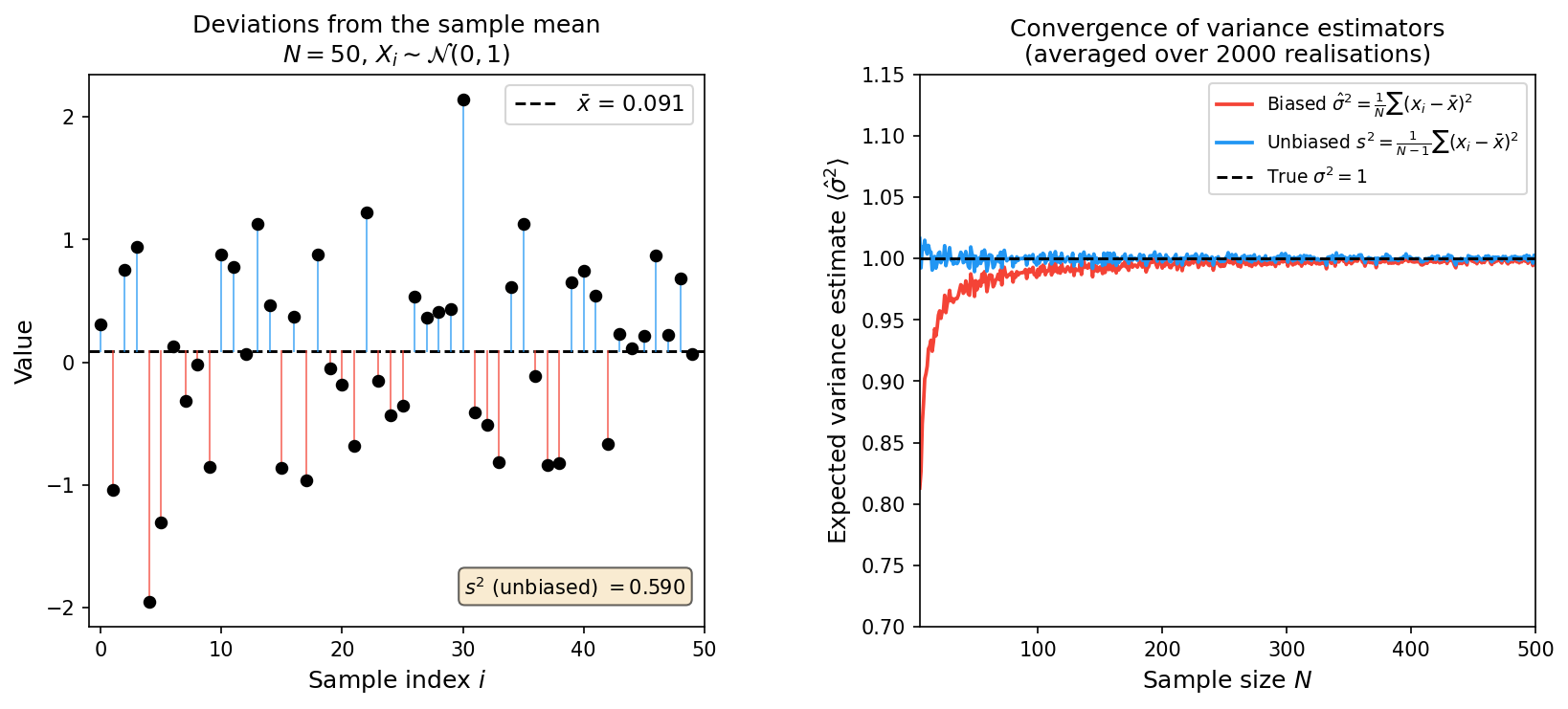
Figure / in-class demonstration
Run variance_example.py to generate this figure.
The sample standard deviation is defined as:
The variance is the second moment about the mean.
The division by \(N-1\) is required to obtain an unbiased estimate of the true population variance. The bias creeps in because we have to estimate the sample mean to get the sample variance, and so we lose one of our degrees of freedom (more on this later). Another way to see this is:
What we want is the first term, and the second term is our bias. You can show that adding the \(N-1\) gets rid of the low bias of the variance, but we don’t go into that derivation here. In practice, if using \(N\) or \(N-1\) matters in your analysis, you are in trouble anyway.
The mean is the average picture (stationary picture), while the variance describes all the interesting wiggles and variability about the mean.
The estimate of the variance depends greatly on the sample rate (e.g. if you are using daily data, monthly data, yearly data, etc).
Also, one can show that two time series with the same variance (say, of 1) but with different persistences can give different answers depending on the sample window (how long of the record you look).
Higher moments#
In general, all moments are defined as:
\(m_2\) is the variance; \(m_3\) is the skewness; \(m_4\) is the kurtosis.
These can also be given in non-dimensional form as:
where \(s\) is the sample standard deviation.
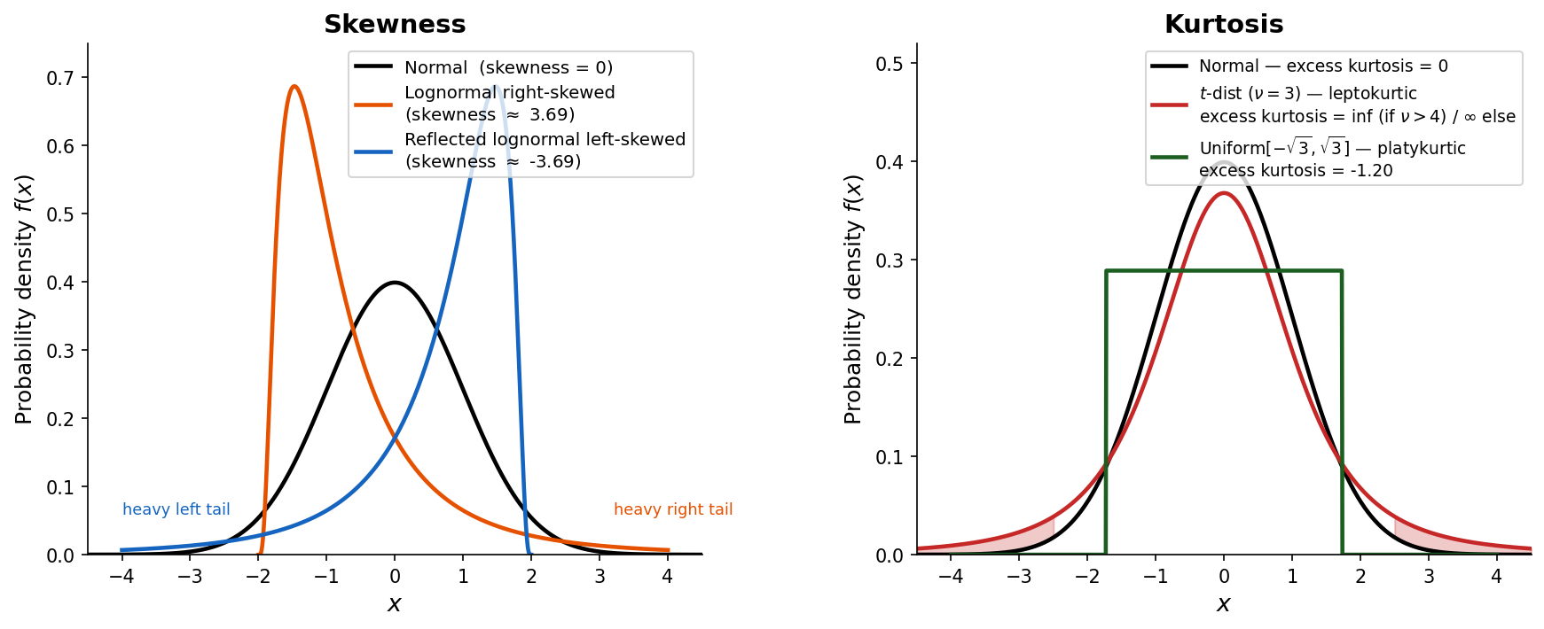
The skewness indicates the degree of asymmetry of the distribution about the mean. \(a_3 > 0\) indicates a long tail on the positive side of the mean (a Gaussian has \(a_3 = 0\)).
The kurtosis indicates the degree of peakedness of the distribution. \(a_4 > 3\) indicates a more peaked distribution compared to a Gaussian, which has \(a_4 = 3\).
Figure / in-class demonstration
Run skewness_kurtosis.py — the left panel illustrates skewness, the right panel kurtosis.
Typically, higher order moments are given in terms of the standardized units, for ease of comparison (and so units don’t matter).
Basic probabilities; unions; intersections; conditional probabilities; Bayes theorem#
Probabilities: Unions & Intersections#
Define some event, \(E\), for example, \(E\) is that you roll a die and get a 2.
For a fair die, we write that the probability of \(E\):
The probability of not \(E\) happening, or,
For the case of rolling the die,
The probability that two events, \(E_1\) (rolling a 5) and \(E_2\) (rolling a 6) will both occur is called the intersection of the two probabilities and is written
The probability that either or both of two events, \(E_1\) (rolling a 5) and \(E_2\) (rolling a 6) will occur is called the union of the two probabilities. This is written
One can see why the intersection term comes into the union equation by drawing a Venn Diagram.
Figure / in-class demonstration
Run venn_diagram.py
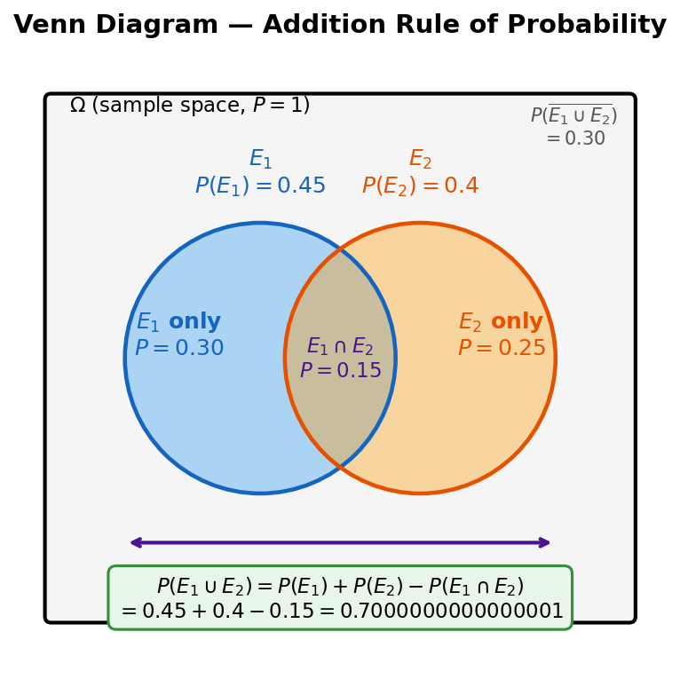
In this diagram the area in the rectangle represents the total probability of one, and the area inside the two event circles indicates the probability of the two events. The intersection between them gets counted twice when you add the two areas and so must be subtracted to calculate the union of the probabilities. If the two events are mutually exclusive, then no intersection occurs, i.e., if one happens, we know the other did not happen at that time.
Another important concept is conditional probability,
read “\(E_2\) given \(E_1\)”.
Changing this conditional probability relationship around a little yields a formula for the probability that both events will occur, called the multiplicative law of probability:
If \(E_1\) and \(E_2\) are independent events (their probabilities don’t depend on one another, like rolling a die), then
and thus
This is the definition of statistically independent.
Rolling a fair die yields statistically independent events, and thus, the probability of rolling both a 5 and a 6 is equal to \(\frac{1}{6} \cdot \frac{1}{6} = \frac{1}{36}\).
Note, if the two events are not independent, multiplying the probabilities will give the wrong answer!
Example of conditional probability
Say the probability of it raining on Monday is 60%. But, you know from looking at historical records that the probability of it raining the day after it rains is 80% (it is more likely than not to rain the day after it rains). So, whether it rains on Tuesday is dependent on whether it rains on Monday. What is the probability it will rain Monday and Tuesday?
Bayes Theorem#
Let \(E_i, i = 1,2,3\dots N\) be a set of \(N\) events such that the set \(E_i\) includes all possible possibilities in a set \(S\) and the events are mutually exclusive. Then, for any event \(B\), with \(\Pr(B) > 0\)
Note that since the \(E_i\)’s cover all possible outcomes, the following is true:
Note that this is the denominator in Bayes theorem.
A useful relation when doing Bayes Theorem problems is the following:
In general, Bayes’ Theorem takes \(\Pr(A \mid B)\) and turns it into \(\Pr(B \mid A)\).
Let’s do an example.
Example of Bayes Theorem: testing for a chemical
You have designed a test which tells whether a sample of air has a harmful airborne chemical or not. The probability that any individual sample has the chemical is 1/1000. The test never gives a false negative result (saying that the sample does not have the chemical, when in fact it does). The chance of a false positive is also small, say 5%. If you test a sample of air today and the test comes back positive, what is the probability that the chemical was actually in the sample?
Your instincts might tell you 95%, since the false positive rate is 5%. However, this is not correct, since you need to take into account all of the information. To do these problems, it is good to follow these steps:
Define your variables
Clearly state what you want to know
List all of the information the problem gives you
Check the assumptions for your method of solving
Then, solve for what you listed in Step 2
(1) Define the variables:
(2) State what we want to know:
(3) List what we know:
(4) Check assumptions. Here, the set \(S\) is made of two possibilities that span all possibilities,
(5) We can now apply Bayes Theorem.
We know all values, except \(\Pr(+ \mid C)\). However, this is equal to
Plugging in the values leads to \(\Pr(C \mid +) = \frac{1}{51} \approx 2\%\). This result shows how important it is to take into account the background rate — otherwise, you may have thought the probability was 95%, not 2%.
Example of Bayes Theorem: cab accidents
The next problem comes from Chapter 16 of “Thinking Fast and Slow” by Daniel Kahneman, a popular science book on how our brains process information.
A cab was involved in a hit and run accident at night. Two cab companies, the Green and the Blue, operate in the city. You are given the following data:
85% of the cabs in the city are Green and 15% are Blue.
A witness identified the cab as Blue. The court tested the reliability of the witness under the circumstances that existed the night of the accident and concluded that the witness correctly identified each one of the two colors 80% of the time and failed 20% of the time.
What is the probability that the cab involved in the accident was Blue rather than Green?
Your instincts might tell you 80% — but then you wouldn’t be taking into account the background rate of the cabs in the city.
Note that if there hadn’t been a witness, your answer would have been 15% (this is a frequentist approach — more on this later).
(1) Define the variables:
(2) State what we want to know:
(3) List what we know:
(4) Check assumptions: OK.
(5) Solve for what you listed in Step (2): Apply Bayes Theorem for \(\Pr(B \mid W)\).
Example of Bayes Theorem: Monty Hall problem
This is a famous one, called the Monty Hall Problem and loosely based on a gameshow called “Let’s Make A Deal” with host Monty Hall.
Suppose you’re on a game show, and you’re given the choice of three doors (A, B, C): Behind one door is a car; behind the others, goats (and you don’t like goats). You pick a door, say door A, and the host, who knows what’s behind the doors, opens another door, say door B, which has a goat.
Monty then says to you, “Do you want to switch your choice and pick door C?” Is it to your advantage to switch your choice?
To start, imagine there is no host, and you have to choose the door with the car. You choose door A, what is the probability that you are correct? Easy — \(\frac{1}{3}\).
Monty showing you what is behind one of the doors is extra information. This should tell you, perhaps use Bayes Theorem! (Drawing pictures can help too.) The hardest part of this problem is figuring out how to set it up.
Without loss of generality, we will assume that you have chosen door A.
(1) Define the variables:
(2) State what we want to know:
(3) List what we know:
(4) Check assumptions. OK.
(5) We can now apply Bayes Theorem.
So, if you switch your choice, you have a higher probability of winning the car!
Probability philosophy#
There are two general philosophies of thought on statistics: (a) frequentist approach, and (b) the Bayesian approach.
Frequentist: if you give an event many opportunities to occur, the probability of occurrence is the
This approach works well when you can repeat an experiment many, many times. In more detail:
any given experiment can be considered as one of an infinite sequence of possible repetitions
probability is seen as the “potential frequency of an outcome”
the result is often a “true or false” conclusion from a significance test
it answers the question “how likely is my data if the null hypothesis is true?”, that is, \(\Pr(\text{data} \mid \text{null hypothesis})\)
Bayesian: this approach is named after the frequent use of Bayes theorem, which takes into account a priori information that may not be useable by a frequentist. In more detail:
the evidence about the true state of the world is expressed in terms of degrees of belief
any probability is a conditional probability given what one knows (varies from person to person)
probability is seen as the “plausibility of an outcome”
it “updates” a prior hypothesis when new information comes to light
it answers the question “how likely is it that a hypothesis is true given my data?”, that is, \(\Pr(\text{hypothesis} \mid \text{data})\)
The last bullet in each list is the entire disagreement compressed into one line: a frequentist reports \(\Pr(\text{data} \mid H)\), whereas a Bayesian reports \(\Pr(H \mid \text{data})\). Bayes’ theorem is precisely the bridge between the two, which is why it sits at the centre of this debate.
Often, these two approaches can give different answers:
For example, in the Monty Hall problem, we wanted to know the probability that the car was behind a certain door, say door C. A frequentist approach would be to say, if I run this experiment thousands of times, how often will the car be behind door C? The answer is \(1/3\) of the time.
In our Bayesian formulation, we used additional a priori information, namely, that Monty Hall showed us that it wasn’t behind a certain door. A frequentist approach does not use this information, while a Bayesian approach does.
For the cab accident example, a frequentist would say the probability of the cab in the accident being Blue is 80%, the probability the witness was correct. The Bayesian approach, however, also took into account the background rate of the number of cars in the city, information that the frequentist approach couldn’t use.
Worked comparison: “Was 2025 the warmest year on record?”
The two philosophies differ in more than just whether prior information is used. The deeper split is over what kind of thing is allowed to carry a probability. The cleanest way to see this is to hand both approaches the same numbers and watch them produce different sentences.
The setup. Global-mean surface temperature is not measured perfectly: the station network is uneven, instruments drift, and the ocean is sparsely sampled. Suppose an analysis centre reports
The uncertainty on the gap, \(\sigma_d\), is smaller than the uncertainty on either year alone, because both years are estimated from the same station network and much of the error cancels in the difference. Both camps accept these numbers. They disagree about what may be said next.
The frequentist. The true 2025 anomaly is a fixed physical constant. The event “2025 was the warmest year” already happened, exactly once — it is either true or false, and its probability is \(0\) or \(1\); we simply don’t know which. Since it is not repeatable, a frequentist declines to attach a probability to it at all, and instead makes a statement about the measurement procedure:
If the two years were truly tied (\(d_{\text{true}} = 0\)), then measurement noise alone would produce an apparent gap of \(0.04^\circ\)C or larger in magnitude about 42% of the time.
(From \(z = 0.04/0.05 = 0.8\); we formalise this kind of calculation later under hypothesis testing.) The conclusion: the observed gap is comfortably within what noise alone generates, so the data do not establish a new record. Note where the probability sits — on the data, given a hypothesis: \(\Pr(\text{data} \mid H)\).
The Bayesian. The quantity \(d = \mu_{2025} - \mu_{2024}\) is simply unknown, and probability measures how strongly the evidence pins it down. With a flat prior — no reason beforehand to favour either year — the posterior is centred on the observed gap:
Given the observations, there is a 79% probability that 2025 was the warmest year on record.
Here the probability sits on the hypothesis, given the data: \(\Pr(H \mid \text{data})\).
Same data, two headlines.
Frequentist |
Bayesian |
|
|---|---|---|
What is random? |
the data |
the unknown quantity |
Can “2025 was warmest” have a probability? |
No — it is a fixed fact |
Yes — it is an unknown |
The statement produced |
“noise alone would fake a gap this big 42% of the time” |
“79% probability 2025 set a record” |
Form of the answer |
\(\Pr(\text{data} \mid H)\) |
\(\Pr(H \mid \text{data})\) |
Why both numbers are correct. 42% and 79% are not in conflict; they are answers to different questions. In fact they are arithmetically linked: \(1 - 0.79 = 0.21\), which is exactly half of \(0.42\). With a flat prior and Gaussian errors, the Bayesian posterior and the one-sided frequentist calculation land on the same number. What never coincides is what the number is a probability of.
The practical lesson. Whenever you hear “there is a 95% chance the true value lies in this range,” that is a Bayesian sentence — even when the interval was produced by frequentist machinery. Misreading frequentist output as a probability statement about the truth is the single most common error in applied statistics, and we will return to it when we construct confidence intervals.
Bayes Theorem is actually used quite often in atmospheric science in the form of the Kalman Filter, for example, for forecasts. At its base level, the Kalman Filter is an iterative application of Bayes Theorem which uses uncertainties in measurements to weigh their use when updating the next time step.
Tying it together: Moments, PDFs, and Bayes’ Theorem#
With the rules of probability and Bayes’ theorem now in hand, we can close the loop back to the moments introduced at the start of this section. The key insight is that the PDF \(f(x)\) — which we have been using to define probabilities — is also the object that gives every moment its precise population definition.
Moments as expectations over a PDF#
Earlier we defined moments using the sample formula \(m_r = \frac{1}{N}\sum_i (x_i-\overline{x})^r\). Now that we have introduced the probability density function \(f(x)\), we can express the same quantity in population (continuous) form — every moment is simply an expectation weighted by \(f(x)\):
This integral is the continuous analogue of \(\frac{1}{N}\sum_i(x_i-\mu)^r\): instead of averaging over a finite list of data points, we integrate over all possible values of \(x\), weighted by how probable each value is under \(f(x)\). The table below shows how the familiar statistics fall out of this single formula:
\(r\) |
Moment |
Population expression |
|---|---|---|
1 |
Mean (about zero) |
\(\mu = \int x\,f(x)\,dx\) |
2 |
Variance |
\(\sigma^2 = \int (x-\mu)^2 f(x)\,dx\) |
3 |
Skewness (non-dim.) |
\(a_3 = \int (x-\mu)^3 f(x)\,dx \;/\;\sigma^3\) |
4 |
Kurtosis (non-dim.) |
\(a_4 = \int (x-\mu)^4 f(x)\,dx \;/\;\sigma^4\) |
Key takeaway: the PDF \(f(x)\) encodes all information about a distribution; every moment is a specific weighted integral of it. The Gaussian is special in that knowing only \(\mu\) and \(\sigma^2\) (the first two moments) completely determines \(f(x)\) — which is why so much of statistical inference focuses on these two quantities.
From the product rule of probability to Bayes’ theorem#
We derived the multiplicative law of probability above:
For two continuous random variables \(X\) and \(Y\), the exact same factorisation applies to their joint PDF:
What does this equation actually say physically?
Both sides of \(f(x \mid y)\,f(y) = f(y \mid x)\,f(x)\) are just two different ways to write the same joint probability: the chance that the true temperature is \(x\) and the sounding reads \(y\) simultaneously.
Think of it like asking: “what is the probability that it rains AND you carry an umbrella?” You could compute it two ways:
Both routes give the same joint probability — they are just different orderings of the same story.
Back to the radiosonde example, \(x\) = true temperature, \(y\) = sounding reading:
Left side — \(f(x \mid y)\,f(y)\): start from the observation, work toward the truth
\(f(y)\): how often does the sounding read \(-17°\)C? (averaged over all possible true temperatures)
\(f(x \mid y)\): given the sounding read \(-17°\)C, what is the probability the true temperature is \(x\)?
Together: the chance that the sounding reads \(-17°\)C and the true temperature is \(x\) = (evidence) × (posterior)
Right side — \(f(y \mid x)\,f(x)\): start from the truth, work toward the observation
\(f(x)\): how probable is it that the true temperature is \(x\)? (the model forecast)
\(f(y \mid x)\): if the true temperature were \(x\), how likely would the instrument read \(-17°\)C?
Together: the chance that the true temperature is \(x\) and the sounding reads \(-17°\)C = (prior) × (likelihood)
The equation is therefore not saying anything deep — it is just the observation that you can count joint occurrences in either order. Bayes’ theorem follows immediately by dividing both sides by \(f(y)\) to isolate \(f(x \mid y)\) — the posterior you actually want.
Setting the two right-hand sides equal and solving for \(f(x \mid y)\) immediately gives Bayes’ theorem in continuous form:
The four terms map directly onto the Bayesian language introduced above:
Term |
Name |
Role |
Atmospheric example |
|---|---|---|---|
\(f(x)\) |
Prior |
belief about the true state \(X\) before seeing any data |
Yesterday’s model forecast says the true 500 hPa temperature over Colorado is probably around \(-20°\)C, with some spread reflecting forecast uncertainty |
\(f(y \mid x)\) |
Likelihood |
if the true state were \(x\), how probable would it be to observe \(y\)? |
The radiosonde has a known instrument error of ±2°C — so if the atmosphere truly is at \(-20°\)C, there is a high chance the sounding reads near \(-20°\)C and a low chance it reads far from it. We ask this for every possible true temperature \(x\), not just the model value |
\(f(x \mid y)\) |
Posterior |
updated belief about the true state after observing \(Y=y\) |
The sounding actually reads \(-17°\)C; combining this with the forecast gives a refined estimate of the true temperature — somewhere between \(-20°\)C and \(-17°\)C, weighted by how much we trust the model vs. the instrument |
\(f(y)\) |
Evidence |
normalising constant ensuring the posterior integrates to 1 |
The overall probability of getting a \(-17°\)C reading, averaging over all temperatures the atmosphere could plausibly be at; keeps the posterior a proper probability distribution |
Connecting the continuous and discrete forms
The discrete Bayes formula used throughout the examples above,
is simply the continuous formula with integrals replaced by sums and PDFs replaced by probability masses. The correspondence with the table above is:
Discrete |
Continuous |
Role |
Radiosonde example |
|---|---|---|---|
\(E_j\) |
\(x\) |
the true (unknown) state — what you want to infer |
the true 500 hPa temperature |
\(B\) |
\(y\) |
the observation — the data you actually have |
the radiosonde reading |
\(\Pr(E_j)\) |
\(f(x)\) |
Prior |
model forecast distribution |
\(\Pr(B \mid E_j)\) |
\(f(y \mid x)\) |
Likelihood |
instrument error model |
\(\Pr(E_j \mid B)\) |
\(f(x \mid y)\) |
Posterior |
updated temperature estimate |
\(\sum_i \Pr(B \mid E_i)\Pr(E_i)\) |
\(\int f(y\mid x)\,f(x)\,dx\) |
Evidence \(f(y)\) |
normalising constant |
In short: \(E_j\) is the hypothesis about the true state (plays the role of \(x\)), and \(B\) is the observed evidence (plays the role of \(y\)). The discrete sum over all possible \(E_i\)’s is just the finite analogue of integrating out \(x\) over all possible true states.
Worked example: Gaussian prior × Gaussian likelihood → Gaussian posterior#
Suppose the true signal \(X\) has a Gaussian prior and the observation \(Y\) is the signal corrupted by Gaussian noise:
Since the evidence \(f(y)\) does not depend on \(x\), we only need the posterior up to a normalising constant:
Taking the log and collecting all terms in \(x\):
Completing the square in \(x\) identifies this as a Gaussian \(\mathcal{N}(\mu_1, \sigma_1^2)\) with:
Physical interpretation
Precisions add. Each source of information (prior, observation) contributes its own precision \(1/\sigma^2\); the posterior is always sharper than either input alone (\(\sigma_1 < \sigma_0\) and \(\sigma_1 < \sigma_w\)).
Posterior mean is a precision-weighted average of the prior and the observation:
Noisy instrument (\(\sigma_w \gg \sigma_0\)): posterior hugs the prior \(\mu_0\).
Diffuse prior (\(\sigma_0 \gg \sigma_w\)): posterior is pulled strongly toward the observation \(y\).
Link to moments: because the posterior is Gaussian, \(\mu_1\) is simultaneously the mean, mode, and median of the posterior — and it minimises the posterior mean-squared error. This connects Bayesian inference back to the sample statistics (\(\overline{x}\), \(s\)) introduced at the start of this section.
Link to the Kalman Filter. This two-Gaussian update is exactly one step of the Kalman Filter introduced above. The prior at step \(k\) is the Gaussian model forecast; the likelihood is the Gaussian observation error; the posterior is the analysis that initialises the next forecast cycle.
With moments expressed as PDF-weighted integrals and Bayes’ theorem derived from the product rule of joint PDFs, we now have a unified probabilistic language. Before moving to significance testing, it is worth making the connection to atmospheric data assimilation explicit — because the Gaussian × Gaussian result above is data assimilation, just written in statistician’s language.
Data assimilation as Bayes’ theorem (optional reading)#
The scalar case. The worked example gave a posterior mean:
In data assimilation (DA), the identical equation is written as:
The term-by-term translation between the two languages is:
Bayes / stats |
DA notation |
Meaning |
|---|---|---|
Prior mean \(\mu_0\) |
Background \(x^b\) |
Model forecast |
Prior variance \(\sigma_0^2\) |
Background error variance \(\sigma_b^2\) |
Uncertainty in the forecast |
Observation \(y\) |
Observation \(y^o\) |
What the instrument reads |
Obs. noise variance \(\sigma_w^2\) |
Observation error variance \(\sigma_o^2\) |
Uncertainty in the instrument |
Posterior mean \(\mu_1\) |
Analysis \(x^a\) |
Best estimate of the true state |
Posterior variance \(\sigma_1^2\) |
Analysis error variance \(\sigma_a^2\) |
Remaining uncertainty after assimilation |
Precision-weighted blend |
Kalman gain \(K\in[0,1]\) |
How much to trust obs. vs. forecast |
The Kalman gain controls the blend:
\(K \to 0\) when \(\sigma_o^2 \gg \sigma_b^2\): the instrument is noisy → stay close to the forecast.
\(K \to 1\) when \(\sigma_b^2 \gg \sigma_o^2\): the forecast is uncertain → pull strongly toward the observation.
The multivariate extension. In practice the true state is a vector \(\mathbf{x}\) (millions of model grid points) and observations \(\mathbf{y}^o\) are scattered in space and may not sit on the model grid. The scalar Bayes update generalises directly to matrices:
where:
Symbol |
Name |
Generalises |
|---|---|---|
\(\mathbf{B}\) |
Background error covariance matrix |
scalar \(\sigma_b^2\) |
\(\mathbf{R}\) |
Observation error covariance matrix |
scalar \(\sigma_o^2\) |
\(\mathbf{H}\) |
Observation operator |
maps model state → what instrument would see (e.g. integrates a temperature profile to simulate a satellite radiance) |
\(\mathbf{y}^o - \mathbf{H}\mathbf{x}^b\) |
Innovation (or departure) |
the “surprise” — how much the observation disagrees with the forecast |
The iterative picture — Kalman Filter as sequential Bayes. Applying this update repeatedly in time gives the Kalman Filter:
Each forecast–update cycle is one application of \(f(x\mid y) \propto f(y\mid x)\,f(x)\). The posterior at step \(k\) becomes the prior at step \(k+1\).
The cost-function view (3D-Var / 4D-Var). Instead of computing the full posterior, operational centres often find the maximum a posteriori (MAP) estimate — the state \(\mathbf{x}\) that maximises \(f(\mathbf{x}\mid\mathbf{y}^o)\), equivalently minimises \(-\ln f(\mathbf{x}\mid\mathbf{y}^o)\):
Minimising \(J\) is the 3D-Var problem used operationally at weather centres (ECMWF, NCEP, etc.). The two terms map directly onto the prior and likelihood in Bayes’ theorem — it is simply finding the mode of the posterior in log-space. 4D-Var extends this by integrating the model forward in time inside the cost function, allowing observations at multiple times to constrain the initial state simultaneously.
Summary: Bayes → DA dictionary
The progression from the scalar Gaussian example to operational data assimilation is one of generalisation, not of new ideas:
Scalar Bayes (worked example above) → analysis of a single variable at one point
Kalman Filter → scalar Bayes applied repeatedly in time
Multivariate Kalman Filter → extends to full model state vector \(\mathbf{x}\)
3D-Var / 4D-Var → finds the MAP estimate of \(\mathbf{x}\) by minimising the negative log-posterior \(J(\mathbf{x})\)
Ensemble Kalman Filter (EnKF) → estimates \(\mathbf{B}\) from an ensemble of model runs rather than assuming it is fixed; widely used in atmospheric and oceanic data assimilation today
All of these are Bayes’ theorem, applied to the problem of estimating the true atmospheric state from a combination of model forecasts and noisy observations.
Statistical Significance Testing#
Normal distribution#
The probability of an event occurring between \(a\) and \(b\) is:
where \(f(x)\) is the probability density function (PDF). Note that for continuous \(f(x)\):
\(f(x)\) must have the following characteristics to be a probability density function:
\(f(x) \geq 0\) for all \(x\)
\(\int_{-\infty}^{\infty} f(x) = 1\)
The cumulative density function (CDF) at value \(b\) is denoted \(F(b)\) and is the probability that \(x\) assumes a value less than \(b\):
hence,
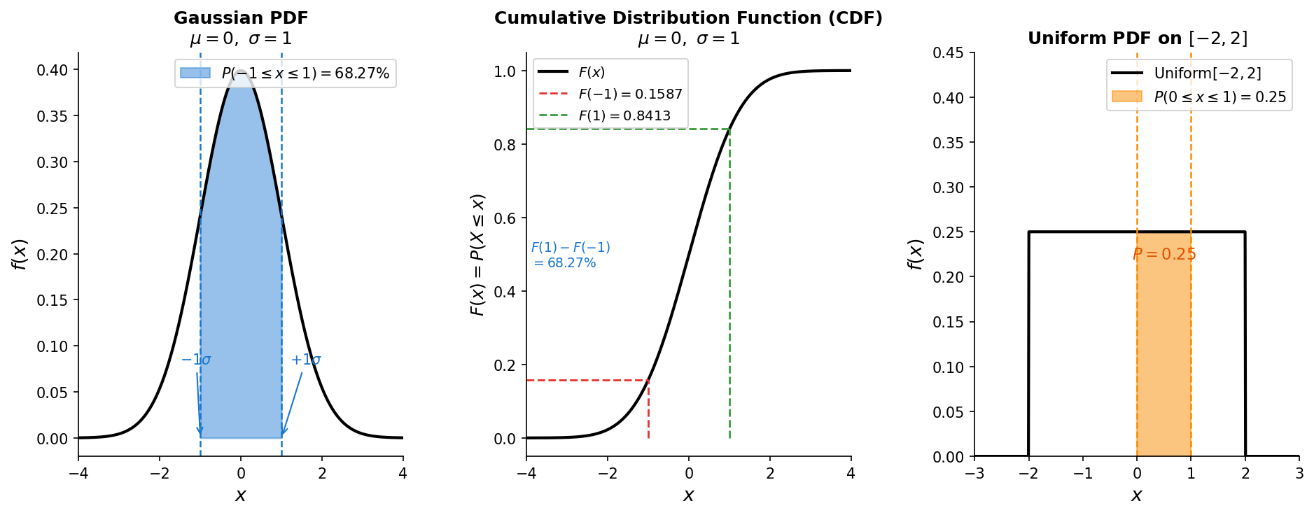
Figure / in-class demonstration
Run what_is_pdf.py
The probability density function for a variable \(x\) that is normally distributed about its mean is given by:
The associated cumulative distribution function is given as:
The probability that \(x\) will fall between two values \(a\) and \(b\) is thus:
Often, one standardizes the normal distribution by defining a variable \(z\):
Note that in this case, the mean of \(z = 0\) and the standard deviation of \(z = 1\). This is very useful for discussing properties of the normal distribution with others who may have variables with different means and standard deviations. For example, recall in the discussion of skewness and kurtosis, the standard normal has a skewness of 0 and a kurtosis of 3.
If one standardizes to \(z\), then
(note that the \(\sigma\) no longer appears in the denominator due to the transformation of \(F(z)\) using \(z = (x-\mu)/\sigma\) and needing to replace \(dx\) with \(\sigma \cdot dz\))
Figure / in-class demonstration
Run normal_distribution.py — the left panel compares a sample histogram with the theoretical PDF, while the centre and right panels show the two-tailed and one-tailed regions used just below.
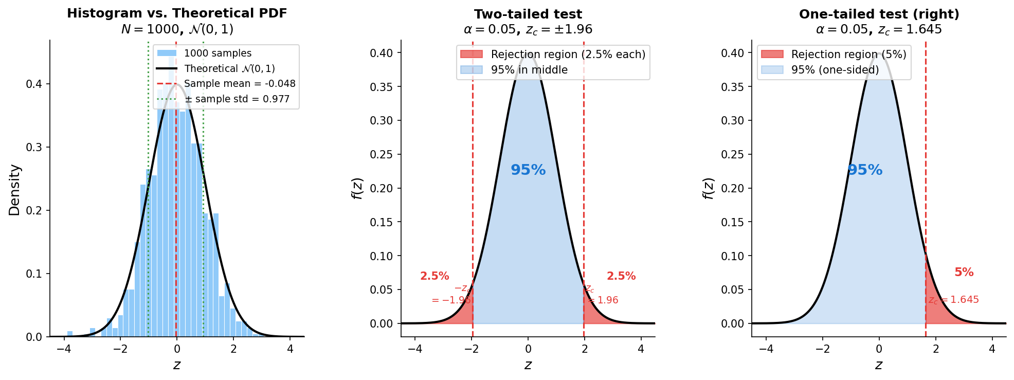
Recall that \(z\) is a standardized normal variable, and so, \(z=2\) is \(z=2\) standard deviations. Thus, there is a 4.55% probability that \(z\) will fall outside of 2 standard deviations of its mean (two-tailed probability) and a 2.275% chance it will exceed \(+2\) standard deviations (one-tailed probability). These two cases are exactly the centre and right panels of the figure above.
Statistical Significance Testing: the t-statistic and z-statistic#
Many geophysical variables are normally distributed — so often we can use the normal distribution to test if our sample is different from the population mean. However, always check that our data is normal! Rain rate, for example, is not!
Figure / in-class demonstration
Figure Example: Introduce z-table — hand-out table to class
Using the z-score#
Example
Assume you have 50 years of monthly ENSO indices (\(Z\)), and that the index is well approximated by a standard normal:
Using the table, what is the probability that a randomly chosen month has an ENSO index of exactly \(+2\)?
0%Using the table, what is the probability that a randomly chosen month has an ENSO index of \(+2\) or greater?
\(1-.9772 = 2.08\%\)What is the probability the ENSO index is 1.23 or smaller?
\(0.8907 = 89.07\%\)What is the probability the ENSO index is 1.23 or greater?
\(1-0.8907 = 10.93\%\)What ENSO index gives \(\Pr(Z > \cdot) = 0.1\)?
1.285What ENSO index gives \(\Pr(Z \leq \cdot) = 0.9\)?
1.285What ENSO index gives \(\Pr(Z \leq \cdot) = 0.1\)?
\(-1.285\), use symmetryWhat ENSO index gives \(\Pr(|Z| > \cdot) = 0.1\)?
1.645 and \(-1.645\)
Some useful values,
In Matlab, you can use
In IDL, for the standardized normal, you can use
In python, for the standardized normal, you can use
Estimating the statistical significance of the sample mean with the z-statistic#
Thus far, we have covered how to determine the probability of getting a value \(x_i\) within a range \([a,b]\), however, in geophysics, we tend to be more interested in the difference between a sample mean and an underlying population.
We rarely ask, “what is the probability the ENSO index was its value or greater this month?” Instead, we might ask, “Was the ENSO index in 2013 consistent with the climatological behaviour?”
Let \(X = [x_1, x_2, x_3, x_4, \dots, x_N]\) be a random sample of size \(N\) drawn from a normal distribution with population mean \(\mu\) and standard deviation \(\sigma\).
For \(N > 30\), \(\overline{X}\) is normally distributed with,
In other words, the sample mean is an estimate of the population mean, and the error of your estimate (the variance of the distribution of \(\overline{X}\)) decreases as \(N\) increases (as it should). \(\sigma_{\overline{X}}\) is known as the standard error of the mean.
So, how do we test whether the mean of the sample is different from the mean of the population? We can use the z-statistic!
Recall,
Now, we want to test \(\overline{X}\), not \(x\). So, replace \(\mu\) with the population mean of \(\overline{X}\) and \(\sigma\) with the population standard deviation of \(\overline{X}\).
Plugging things in leads to
The z-statistic is now the number of standard errors that the sample mean deviates from the population mean.
We can easily manipulate the equation for the z-statistic to obtain an equation for the difference of two means (as opposed to the difference between a sample mean and the population), where \(\sigma_1\) can be different from \(\sigma_2\):
\(\Delta_{1,2}\) is the hypothesized difference between the two means, which is typically 0 in practice.
Statistical significance of the mean
What is the probability that December 2013 had an ENSO index of 0.50 or greater?
What is the probability that the average 2011–2013 monthly ENSO index was 0.50 or greater assuming that ENSO dynamics have not changed?
(a) Assume the ENSO index is standard normal. \(\mu = 0\), \(\sigma = 1\). Look at table for \(z = 0.50\). \(1-.69 = 31.0\%\). So, not very rare.
(b) Here, we are testing for the sample mean.
The \(\Pr(z > 3.0) \approx 1 - 0.9987 = 0.1\%\).
Such a low probability implies that we had either a very rare event, or, that the dynamics of ENSO changed in 2011–2013 compared to climatological ENSO variability.
Confidence Interval#
Calculating confidence limits
Say we have temperatures for 30 winters with a mean of \(10^{\circ}\)C and a standard deviation of \(5^{\circ}\)C. What is the 95% confidence interval on the true population mean? You may assume that the temperatures are normally distributed.
Since we are interested in the spread about the mean, and since the normal distribution is symmetric about the mean, this can be rewritten as,
Since 95% of the population lies within \(z_{\alpha/2} = \pm 1.96\), it follows that the confidence limit for \(\mu\) is
The 95% confidence interval is defined as the interval that contains the true parameter 95% of the time.
Figure / in-class demonstration
Figure Example: Pass-out handout called Confidence intervals.pdf
Central Limit Theorem#
The arithmetic mean of a sufficiently large number of iterates of independent random variables, each with a well-defined expected value and well-defined variance, will be approximately normally distributed, with standard error of \(\sigma/\sqrt{N}\), where \(N\) is the length of each sample.
This theorem is the basis of most of what we do in statistics, and most of what we do when assessing the significance of geophysical signals.
Figure / in-class demonstration
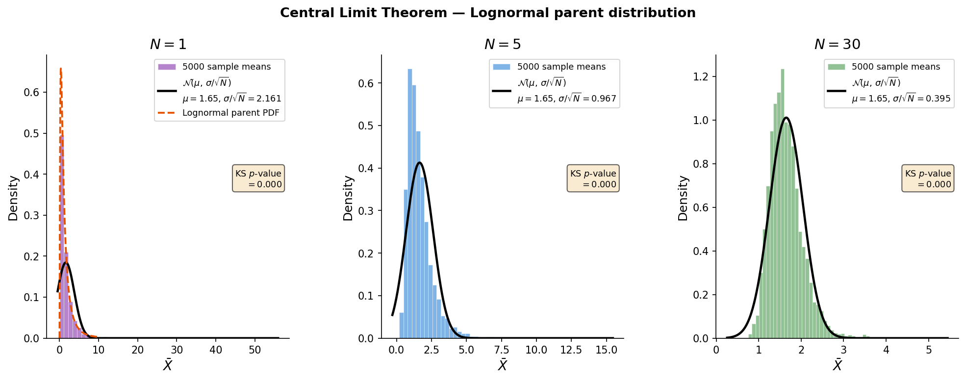
What the central limit theorem says is that if you have a sample that is large enough, you can use the normally distributed z-statistic to estimate probabilities of getting that mean — no matter the distribution of the underlying data.
Rain rate
Rain rates are lognormal (black curve in the Matlab example). Thus, you cannot use the z-statistic to determine, say, the probability of getting a rain rate at any given time of 2 mm/sec. or higher. However, if you want to know the probability of having a monthly average rain-rate of 2 mm/sec. or higher, you can use the z-statistic!
Note, because of the Central Limit Theorem, this is often all people remember from their statistics course — however, be careful, it does not always apply.
The t-statistic: when the sample size is small#
Consider the z-statistic for the sample mean:
To apply this formula, we need to know the \(\sigma\) of the underlying distribution. But often, we don’t know what the underlying distribution is. As we showed in the previous example, if we have a large enough sample, the sample standard deviation \(s\) is a good approximation of the true population \(\sigma\).
However, if \(N < 30\), this is not the case, and the z-statistic does not apply!
In this case, one must use the Student’s t-statistic, introduced by William Sealy Gosset in 1908 to monitor Guinness quality at the brewery in Dublin, Ireland. At the time, he was not allowed to publish anything that he developed while at Guinness, so he used the pseudonym “Student”.
The t-statistic is analogous to the z-score, except it also requires:
The t-statistic is defined as
where \(s\) is the sample standard deviation.
Recall from the Central Limit Theorem example that when \(N \gtrsim 30\), the true standard deviation of the sample means is well approximated by \(s/\sqrt{N}\), and so we can write \(\sigma\). However, in this case, we keep the nomenclature \(s\) since it is unknown what the true \(\sigma\) is.
Note the similarity with the z-statistic:
\(\hat{s}\) is the estimate of the standard deviation based on a limited sample.
If we draw a sample of size \(N\) from a normally distributed population of mean \(\mu\), we find that \(t\) is distributed with the following population density:
\(f_0(\nu)\) is chosen as a normalization factor to make \(\int_{-\infty}^{\infty} f(t)\,dt = 1\).
\(\nu\) is the number of degrees of freedom \(= N-1\). It is the number of independent samples (\(N\)) minus the number of parameters that must be estimated. In the case of the t-statistic, we calculate \(\overline{x}\) and \(s\) but must estimate \(\mu\). Hence, \(\nu = N-1\). More on independent samples later.
Figure / in-class demonstration
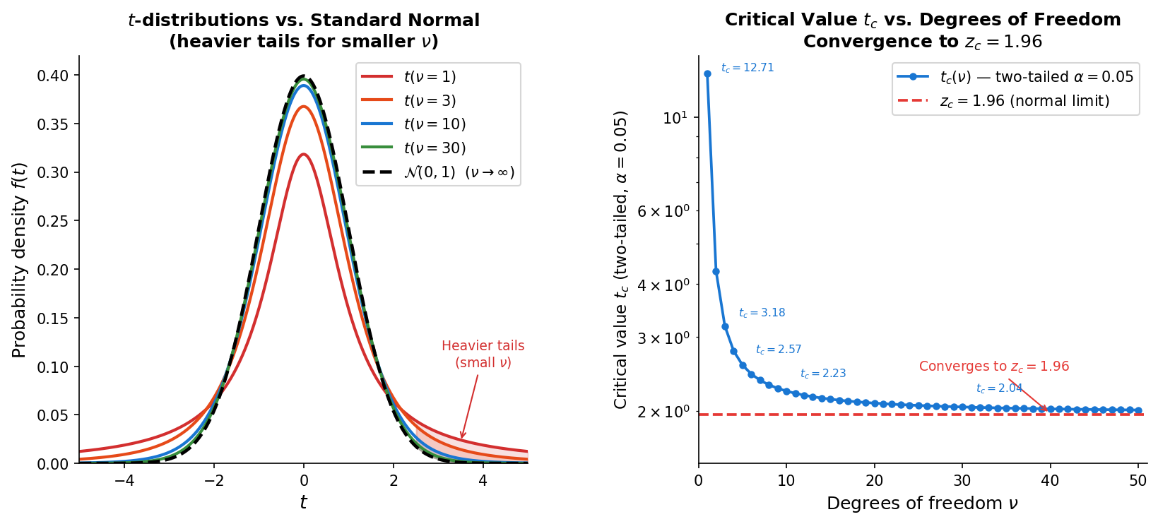
Comparisons between the t-statistic and z-statistic:
most often, the t-distribution is the PDF of the sample means drawn from a normal distribution, but with small \(N\)
unlike the z-stat, the t-stat depends on \(N\) through the degrees of freedom \(\nu\)
smaller values of \(N\) lead to longer tails for the t-stat
as \(N\) increases, the t-stat approaches the z-stat
the key difference is that the t-stat uses an estimate of the standard error based on the sample standard deviation \(s\), instead of the true standard error \(\sigma\)
Confidence intervals for the t-statistic work similarly to the z-statistic,
\(t_c\) is the critical value for \(t\). It depends on the sample size and the significance level desired. You can see values of this statistic in the t-table. Note that it is set up differently than the z-table since it requires a column for \(\nu\).
The difference of means for the t-stat. is very similar to that for the z-stat, but with slight modifications. Assume two samples \(N_1\) and \(N_2\) are drawn from normal distributions whose standard deviations are equal (\(\sigma_1 = \sigma_2\)).
where \(\nu = N_1 + N_2 - 2\) and \(\Delta_{1,2}\) is the hypothesized difference.
The pooled variance \(\hat{\sigma}^2\) is a weighted average of the sample variances.
A similar statistic applies for the z-score, but we use the true sample variances instead:
Comparing the z-stat and t-stat
You have 5 years of monthly-mean temperature data derived from the MSU4 satellite. The mean temperature along 60N during January is \(\sim -60^{\circ}\)C and the standard deviation is \(\sim 8^{\circ}\)C. What are the 95% confidence limits on the true population mean?
z-statistic
The critical value \(z_c = \pm 1.96\) for 95% confidence. Thus, the population mean \(\mu\) is expected to lie within
t-statistic
The critical value \(t_c = \pm 2.78\) for \(\nu = 5-1=4\). (Note: we want to use 0.025 since a two-tailed test.) Thus, the population mean \(\mu\) is expected to lie within
Thus, using the t-statistic gives a wider confidence range than the z-statistic, reflecting the additional uncertainty associated with a small \(N\).
If we erroneously used the z-stat instead of the t-stat, we would underestimate the 95% confidence bounds by 35%.
When to use (and not use) the t-test#
If you are choosing between the z-test and t-test, use the t-statistic! It converges to the z-test for large \(N\).
When applying the t-test, you are implicitly making a very strong assumption: that the underlying distribution is normal.
Always check your normality assumption: plot your data, look at the skewness, kurtosis, etc. There are fancy tests to check for normality, e.g. the Kolmogorov–Smirnov test (kstest in Matlab).
Now, we previously discussed the Central Limit Theorem (CLT), which tells us that for a “large enough” sample size, the distribution of sample means is normal. However, note that the t-test applies for small \(N\) but for underlying normal distributions, whereas the CLT only applies for large \(N\).
Thus, you cannot blindly apply the t-test to test differences in sample means if the underlying distributions are not already normal! This is a common mistake made in our field. It is worth revisiting the central limit theorem figure above with this caveat in mind: convergence to normality is guaranteed only in the limit of large \(N\), and the lognormal parent shown there is still visibly skewed at small \(N\).
A note on the independence on N#
In all of the cases thus far, it has been assumed that the \(N\) samples are independent samples. Often, \(N\) observations of a geophysical variable are not independent, for example, they exhibit either spatial or temporal correlations.
For example, the geopotential height is highly auto-correlated so that each day’s value is not independent from the previous or following days. You cannot improve your ability to know a 5-day wave by sampling every 3 hours instead of every 6. We will discuss this more later on in the course.
Hypothesis Testing#
Terminology and symbology#
Figure / in-class demonstration
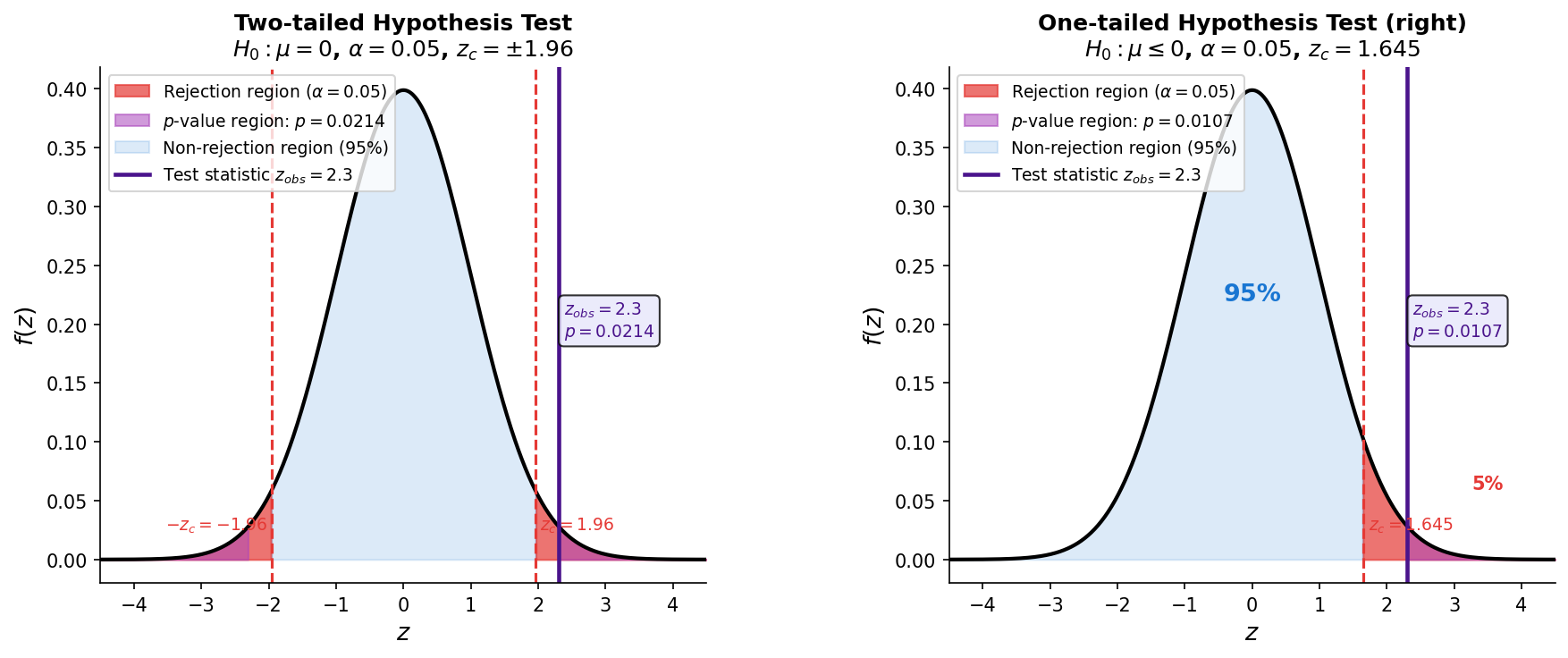
significance/confidence level: \(\alpha\), typically 5% (0.05), often reported as \(1-\alpha\)
critical value: \(t_c\) or \(z_c\), the value that must be exceeded to reject the null hypothesis, one-sided \(t_\alpha\), two-sided \(t_{\alpha/2}\)
p-value: probability of observing an effect given that the null hypothesis is true (probability of your \(t\)-score or \(z\)-score)
Setting-up the problem#
In using statistical significance tests, there are 5 basic steps that should be followed, in order.
State the significance level (\(\alpha\))
State the null hypothesis \(H_0\) and the alternative \(H_1\)
State the statistic to be used, and the assumptions required to use it
State the critical region
Evaluate the statistic and state the conclusion
Proper construction of the null hypothesis and its alternative is critical to the meaning of statistical significance testing.
Usually the null hypothesis is a rigorous statement of the conventional wisdom or a zero information conclusion, and its alternative is an interesting conclusion that follows directly and uniquely from the rejection of the null hypothesis.
Some examples:
\(H_0\): The means of two samples are equal.
\(H_1\): The means of two samples are not equal.
\(H_0\): The anomaly is zero.
\(H_1\): The anomaly is not zero.
\(H_0\): The correlation coefficient is zero.
\(H_1\): The correlation coefficient is not zero.
Hypothesis testing is much weaker than Bayesian statistics (discussed at the beginning of this course). All you are really doing is stating whether the data is consistent with the null hypothesis or not.
You are not saying that the null hypothesis is true, or that the alternative is true, or that either is false.
Example of Hypothesis Testing
Sam went skiing 10 times at Vail this winter. The average temperature on these 10 days was 35F, and their standard deviation was 5F. Sam knows that the climatological mean winter temperature for Vail is 32F. Is this a sign of climate change?
Let’s suppose by a “sign of climate change”, we mean, are the 10 days Sam went skiing sampled from a warmer population than the climatological values? Let’s walk through the 5-steps to answer this question.
Let \(\mu\) be the true mean of the population from which the 10 days Sam went skiing were sampled.
Let’s use 95% confidence (\(\alpha = 0.05\))
\(H_0\): \(\mu = 32^{\circ}\); \(H_1\): \(\mu \neq 32^{\circ}\)
For this problem, we will assume that the temperatures at Vail are normally distributed. Since we have \(N=10\) samples to estimate the true standard deviation (\(\sigma\)) from the sample standard deviation (\(s\)), we must use the t-test.
We will use a two-sided t-test (before he went skiing, Sam didn’t know what to expect from the temperatures). Thus, to reject the null hypothesis we must have \(t > t_{0.025} = 2.262\) (for \(\nu = 9\))
\(t = \dfrac{35-32}{\sqrt{5^2/(10-1)}} = 1.80\)
\(t = 1.80 < t_{0.025}\), so we cannot reject the null hypothesis that the underlying population is different for the days Sam went skiing.
Note, we should not say:
“There was nothing different about the temperatures on the day Sam went skiing.”
…nor…
“There has not been a change in temperatures at Vail over the past few decades.”
We can only say
“The data is consistent with the null hypothesis that the mean of the underlying population on the days Sam went skiing was the same as the climatology.”
…or…
“The higher temperatures present when Sam went skiing are consistent with natural variability.”
Comparison of Means & Hypothesis Testing#
Example
In 2000, you and your science team went into Rocky Mountain National Park to measure the Nitrogen deposition there. You took 17 samples and found they had a sample mean of 30 mg \(\cdot\) N/m\(^2\), and a sample standard deviation of 10 mg \(\cdot\) N/m\(^2\).
In 2014, you repeat your measurements, but this time, due to budget cuts, you are only able to take 7 samples, resulting in a sample mean of 45 mg \(\cdot\) N/m\(^2\) and a sample standard deviation of 20 mg \(\cdot\) N/m\(^2\).
Has Nitrogen deposition significantly increased between 2000 and 2014?
This problem is different than one we have done before, since we are not comparing our sample to a long-term average (or climatology), but we are comparing two sample means to each other. Thus, we need to use a “comparison of sample means” test. The good news is that it is similar to what we have been doing thus far.
Assume two samples \(N_1\) and \(N_2\) are drawn from normal distributions whose true standard deviations are equal (\(\sigma_1 = \sigma_2\)). Then, the t-statistic for sample means is
where \(\nu = N_1 + N_2 - 2\) and \(\Delta_{1,2}\) is the hypothesized difference. The “pooled variance” \(\hat{\sigma}^2\) is a weighted average of the sample variances.
A similar statistic applies for the z-score, but we use the true sample variances instead and they do not have to be equal to each other:
Now, let’s answer the question using hypothesis testing:
95% confidence (\(\alpha = 0.05\))
\(H_0\): \(\mu_{2000} = \mu_{2014}\); \(H_1\): \(\mu_{2000} \neq \mu_{2014}\)
We will use the t-statistic for the comparison of means and we will assume the variance of Nitrogen deposition has not changed, and that it follows a normal distribution (we can check this). We will use a two-sided test since we didn’t know a priori if the difference would be positive or negative.
We will reject the null hypothesis if \(t > t_c = t_{0.025} = 2.0739\) (for \(\nu = 17+7-2=22\)).
Evaluate
\[\begin{split}\begin{aligned} \hat{\sigma} &= \sqrt{\frac{17 \cdot 10^2 + 7 \cdot 20^2}{17+7-2}} = 14.3 \\ t &= \frac{45 - 30 - 0}{14.3\sqrt{\dfrac{1}{17}+\dfrac{1}{7}}} = 2.36 \end{aligned}\end{split}\]Since \(t = 2.36 > t_c\), we can reject the null hypothesis that the sample means in the two years are equal.
Type I and Type II errors#
\(H_0\) is true |
\(H_0\) is false |
|
|---|---|---|
Fail to Reject \(H_0\) |
No Error |
Type II Error (false negative) |
Reject \(H_0\) |
Type I Error (false positive) |
No Error |
The way typical hypothesis tests (frequentist approach) are set up, a 95% confidence level means you have a 5% chance of making a Type I Error, that is, you reject the null hypothesis (think you found something interesting) when you should not have. It is much more difficult to assess the Type II Error — the probability you “play it safe and fail to reject \(H_0\) when something interesting was there”. For typical hypothesis testing, the probability of a Type II error can be very large.
In engineering, you often care about the differences between Type I and Type II errors, and you design your statistics to reflect your judgements. For example, if \(H_0\) is that the bridge will hold up if 10 semi-trucks cross at the same time, and \(H_1\) is that the bridge will not hold up, you might be happier with a Type I Error, which requires that you redesign the bridge, rather than a Type II Error, where you think the bridge will be fine, and it won’t be.
A priori vs. A posteriori#
A priori: you have a reason to expect a relationship ahead of time.
A posteriori: you don’t. This distinction is critical for hypothesis testing.
One-tailed vs. Two-tailed tests:
If you have an “a priori” expectation of the sign of the result, you can use a 1-tailed test. Otherwise, you should use a two-tailed test.
So far, the specific significance levels we have discussed rely on a priori statistics.
Figure / in-class demonstration
Figure Example: Map of correlations with 29040 data points
Gone fishin’ I: a priori vs a posteriori statistics
The jelly bean example on the syllabus (xkcd) shows students testing whether 20 different colors of jelly beans may cause acne, with a significance level of 95% confidence.
Let \(H_0\): jelly beans do not cause acne. What is the probability that 1 jelly-bean color would incorrectly reject \(H_0\) and find a “significant result” by chance alone?
So, our 95% test is really a 36% — we have a 64% chance of finding at least one relationship by chance!
Gone fishin’ II: a priori vs a posteriori statistics
You think that Arctic warming has caused blocking to increase in frequency between the 1980’s and today. You look over the 4 seasons, two latitude bins (north of \(45^{\circ}\)N and south of \(45^{\circ}\)N), and 6 different longitude bins. You test for changes in mean blocking frequency at the 95% confidence level. How many “significant changes” in blocking should you expect by chance alone? How might you apply a posteriori statistics?
You have no a priori knowledge which season or longitude bin should exhibit changes in blocking due to sea ice — thus, you are giving the test \(4 \times 6 \times 2 = 48\) chances to succeed. The number of chances you expect to show significant trends is \(0.05 \times 48 = 2.4\), so, you should find 2.4 “significant changes” by chance alone.
Let \(H_0\): the mean in blocking frequency has not changed.
Thus, your 95% confidence level is really a 9% confidence level!
By trial and error, we can calculate the significance level \(\beta\) for which \(\beta^{48} \approx 0.95\) (our a posteriori statistic). In this case, \(\beta \approx 0.999\). Thus, if we require the blocking changes for each chance to pass at the 99.9% confidence level, then the probability of correctly rejecting the null hypothesis for all chances will be 95%.
Bayesian vs Frequentist approach, revisited#
The two philosophies were introduced earlier, in the Probability philosophy section, where we saw that a frequentist reports \(\Pr(\text{data} \mid H)\) while a Bayesian reports \(\Pr(H \mid \text{data})\). At that point we could only illustrate the distinction with counting arguments. Now that p-values and significance levels are in hand, we can return to it and see what the distinction actually costs in research practice.
The issue is this: a significance test hands you \(\Pr(\text{data} \mid H_0)\), but the quantity you almost always want is \(\Pr(H_0 \mid \text{data})\) — how plausible the hypothesis is, given what you observed. It is tempting to read the first as though it were the second. The two examples below show how badly that substitution can fail when the hypothesis was implausible to begin with, and how Bayes’ theorem repairs it.
Bayesian vs Frequentist approach cont.
You’ve heard the hypothesis that variations in cosmic rays are driving the increase in global-mean temperatures we’ve seen over the last century, but you are very skeptical. You’ve been to a lot of seminars by experts in the field suggesting there is little evidence for this hypothesis. You calculate the correlation between incoming cosmic ray intensity and global-mean temperature and the resulting correlation has a p-value of 0.05. Should you now accept that cosmic rays are the answer and forget about CO\(_2\)?
Frequentist
\(H_0\): there is no real relationship between cosmic rays and global temperature increases
\(H_a\): there is a real relationship between cosmic rays and global temperature increases
p-value \(= 0.05\)
conclusion: if your confidence level is \(\alpha = 0.05\), then you conclude that you can “reject the null hypothesis” that there is no relationship between cosmic rays and the global temperature increase. Note that this approach doesn’t care about \(H_a\), nor does it care about all the evidence against cosmic rays.
Bayesian
\(R\): cosmic rays are driving the increase in global mean temperature
\(\tilde{R}\): cosmic rays are not
\(E\): the evidence obtained from the data, e.g. the correlation
Want: \(\Pr(R \mid E)\)
Know: \(\Pr(E \mid \tilde{R}) = 0.05\)
Bayes’ Theorem:
\[\Pr(R \mid E) = \frac{\Pr(E \mid R)\Pr(R)}{\Pr(E \mid R)\Pr(R) + \Pr(E \mid \tilde{R})\Pr(\tilde{R})}\]Need to know: \(\Pr(E \mid R)\), \(\Pr(R)\) (note that \(\Pr(\tilde{R}) = 1 - \Pr(R)\))
Expert Opinion: \(\Pr(R)\) is your prior probability, what you thought the likelihood that cosmic rays were driving the temperature changes before you analyzed the data. Since you were pretty skeptical due to expert opinion, let’s say \(\Pr(R) = 0.01\) so \(\Pr(\tilde{R}) = 1-.01=.99\).
Expert Opinion: We also need to know \(\Pr(E \mid R)\), that is, the probability of getting the correlation you did if cosmic rays are causing the temperature changes. This one is tricky. For now, let’s say that \(\Pr(E \mid R) = 0.95\), that is, you believe if there was an influence of cosmic rays, you would very likely calculate a correlation as big (or bigger) than what you actually did.
Bayes’ Theorem:
\[\Pr(R \mid E) = \frac{\Pr(E \mid R)\Pr(R)}{\Pr(E \mid R)\Pr(R) + \Pr(E \mid \tilde{R})\Pr(\tilde{R})} = \frac{0.95 \cdot 0.01}{0.95 \cdot 0.01 + 0.05 \cdot 0.99} = 0.16\]Conclusion: you give it a 16% likelihood that cosmic rays are driving the global temperature increase. Put another way, the probability of your null hypothesis being true started off at 99% and now it is still 84% (not 5%)! The likelihood is lower than your p-value because you’ve allowed your prior knowledge to come into the calculation — you thought that the hypothesis was unbelievable (a “rare event”) to begin with. Note that as \(\Pr(E \mid R)\) decreases, \(\Pr(R \mid E)\) decreases as well. For example, if \(\Pr(E \mid R) = 0.5\) (instead of 0.95) you get a likelihood of 9%. If you had no prior knowledge, you would let \(\Pr(R) = \Pr(\tilde{R}) = 0.5\), and you get what you would expect — 95%!
Another Bayesian example
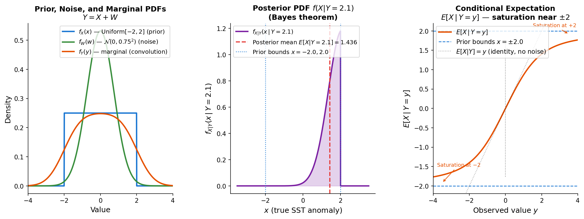
You are interested in measuring the sea-surface temperature off of the Washington coast to within 0.1 units. You know from previous years that the distribution of anomalous sea-surface temperature (denoted as random variable \(X\)) follows a uniform distribution with bounds \((-2,2)\). The problem is that the instrument you use to measure the temperature is known to introduce an additive error. While the exact error during each measurement is unknown, you know from calibration that the error follows a normal distribution with \(\mu=0\) and \(\sigma=0.75\), denoted as \(W\). That is, you measure a random variable \(Y\) that is the sum of the two random variables \(X\) and \(W\): \(Y = X + W\).
You go out and take a measurement and the instrument says that the anomalous sea-surface temperature is \(y = 2.1\). (a) What is the probability that \(X=x\) given that you measured \(y\), or in math, \(\Pr(X=x \mid Y=2.1)\)? (b) For each possible value of \(y\), what is your best estimate of \(x\)?
Frequentist
A frequentist would respond to this information using only the prior distribution, that is, they would respond that the most likely value of \(x\) is the value detected, \(x=y\). They would not take into account the additional information of the known distribution of \(X\) or how \(W\) may modify the signal.
Bayesian
(a) Fig. Figure PDFs shows the distributions of \(X\), \(W\) and \(Y\). Using Bayes’ Theorem, you want to compute the following:
where \(f\) denotes the probability density function.
You know that \(f(X=x)\) follows a uniform distribution, and \(f(Y=y \mid X=x)\) follows the normal distribution of \(W\) but centered on \(\mu=x\) instead of zero. Determining \(f(Y=y)\) is a bit trickier. What you want to know is the distribution of the sum of a normal distribution and a uniform distribution — however, this is not simple to write down analytically. One can determine this distribution using convolution (to be discussed later in the course), model it empirically, or use a built-in software package (e.g. python’s PaCAL). The distribution of \(Y\) is shown in Fig. Figure PDFs. Plugging values into Bayes’ Formula leads to our solution, which is shown in Fig. conditional-PDF figure.
(b) To answer this, you must decide what you mean by “best estimate”. Here, you will define the best estimate based on the posteriori mean. That is, the best estimate of \(X\) given \(Y=y\) is defined by the minimum mean squared error estimate, which is just the expected value of \(X\) given \(Y=y\). In the case of \(Y=y=2.2\), the best estimate is shown as a dashed gray line in Fig. conditional-PDF figure.
Performing this calculation for all possible values of \(y\) leads to Fig. conditional-expectation figure, which shows the most likely sea-surface temperature given that you measure a particular value of \(y\). Note how the curve slowly approaches \(-2\) and \(2\) since \(X\) is bounded by these two values.
Figure / in-class demonstration
Monte Carlo and Resampling techniques#
Monte Carlo and resampling techniques haven’t historically been discussed or used as often because of computational constraints. These days, computer time is cheap and everyone has some, so these techniques can be found more regularly in the peer-reviewed literature.
Resampling techniques: best used when you have a long climatology or control run.
Monte Carlo: useful when you think you know the underlying distribution or behaviour, but you don’t have a long control or climatology — thus, you create many synthetic “realities” to determine the probabilities of certain events.
Why use resampling and Monte Carlo techniques?#
when spatial and temporal correlations are hard to estimate
it is unclear which statistical assumptions are appropriate (e.g. your underlying population is not Gaussian, and the central limit theorem does not apply) — this is when resampling techniques are useful
the statistic of interest does not have a straightforward theory for estimation, but you know the underlying population’s distribution — this is when Monte Carlo simulations are useful
Resampling: bootstrap#
Bootstrapping involves constructing a number of resamples of the original dataset (of equal size to the observed sample of interest) by random sampling with replacement from the original dataset. In this way, you never need to assume anything about the underlying distribution of the data since it is already built into the original dataset. In essence, you ask, by random chance, what is the probability that a particular event (or sample statistic) occurred?
This method is also useful when you are determining statistics other than the mean (e.g. extrema, median, skewness) when we don’t have simple statistics for these variables.
A reference to the bootstrap method is: Efron, B., “Bootstrap Methods: Another Look at the Jackknife”, The Annals of Statistics, Vol. 7, No. 1, pp. 1–26.
The technique is called “bootstrapping” because it almost appears you get something out without putting something in. This is a phrase often used in computer programming to refer to a small amount of simple software that can load more complex software that loads more complex software (etc., etc.), almost as if the program is “pulling itself up by its bootstraps.”
Resampling: jackknife#
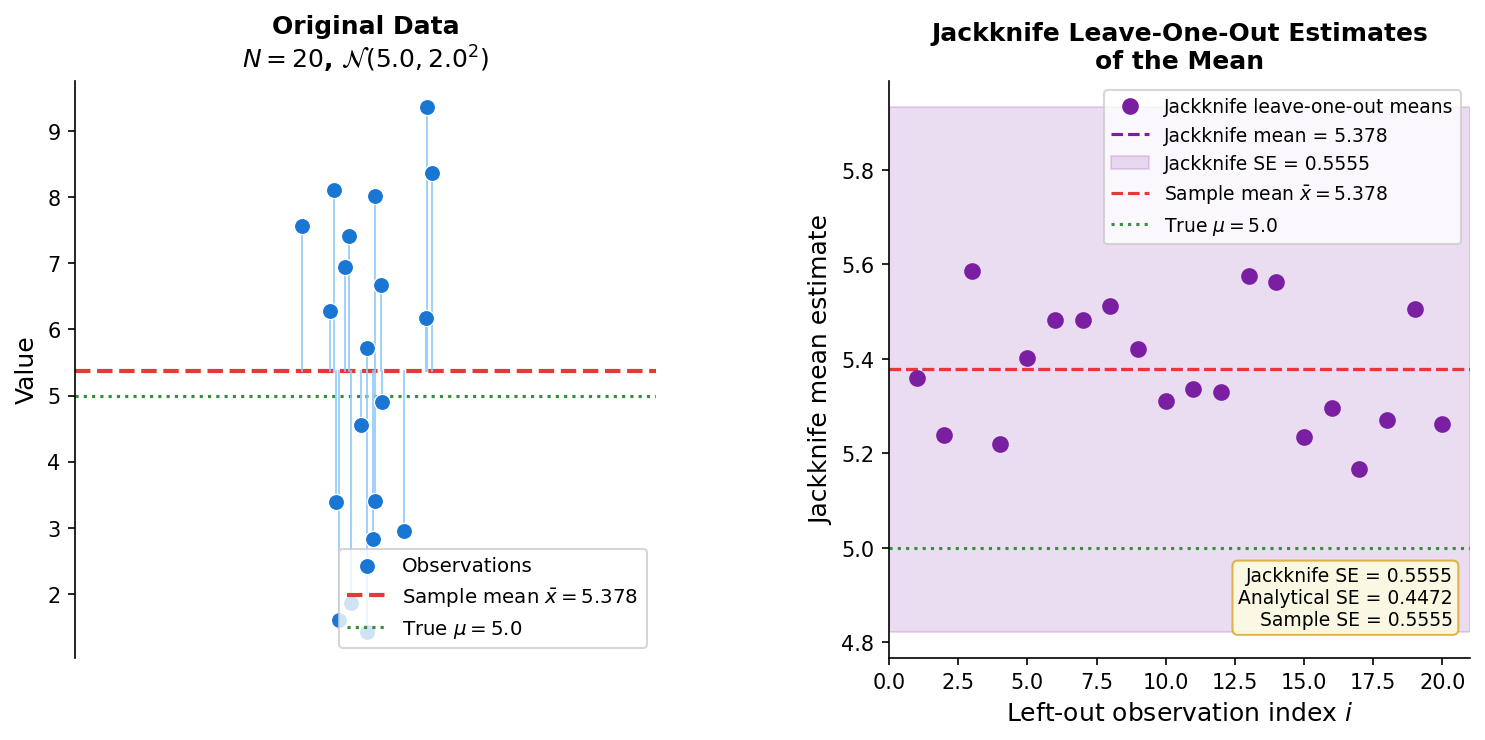
The jackknife method predates the bootstrap method. It is a way of getting error bars (or measuring the variance) of your sample. You systematically remove one value from your sample, and calculate the statistic, then put the value back into the sample and remove the next value, calculate the statistic…and on and on. Then, following a simple formula, you can estimate the variance of the parameter by using the mean of the jackknife estimates of your sample parameter of interest.
You will find the jackknife approach often used to estimate the slope of a line through multiple points, or the y-intercept, etc.
Figure / in-class demonstration
Monte Carlo#
Monte Carlo simulations require that you make an assumption about the underlying distribution. This is useful when you don’t have a large enough base population to perform the bootstrap approach.
The idea is that you create a bunch of synthetic (i.e. fake) data according to your distribution — you create many “realities” based on the same underlying distribution, and then you perform your analysis on these realities to determine the distribution of the statistical parameters of interest.
For example, in Homework 1, you wrote Monte Carlo simulations using the underlying normal distribution.
Resampling: bootstrap
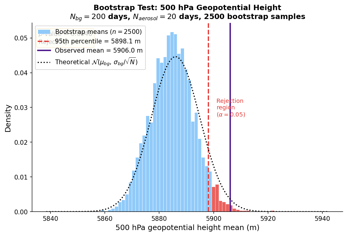
You believe that aerosols grow the most when you have high geopotential heights nearby. You composite the 500 hPa geopotential height on the 20 August days when you have aerosol formation and growth over a site in Egbert, Canada, and you find that the average geopotential on these days is 5900 m. The mean at this station is 5886 m, so the heights are higher. Are these results significant? Or is this just random chance?
Run 2,500 experiments; within each experiment, randomly grab 20 days from the historical geopotential height data, and take the mean of the 20 days. After 2,500 iterations, you will have a distribution of the \(N=20\) sample means under the null hypothesis of random chance. Now, you can look at this distribution and determine the 95% confidence bounds on the \(N=20\) sample means — if the observed value of 5900 m is outside of this range, you have reason to believe it may be more than random chance.
Figure / in-class demonstration
Monte Carlo simulation
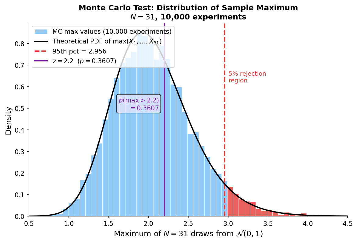
In January (31 days), the maximum daily temperature was 2.2 standard deviations from the climatological mean temperature. If we assume that the daily temperature is normally distributed, how rare is it to have a maximum of \(2.2\sigma\) or greater in 31 daily samples?
We do not have a test for the maximum of a distribution — note, this is not the mean.
We can’t use the bootstrap approach, since we don’t have the population to resample from; we only have our 31 points.
However, since our null hypothesis is that the values come from a standard normal, we can create synthetic data to determine the confidence interval on the maximum in a sample of \(N=31\).
If we had the climatological data (say 50 years of data), we could instead follow a bootstrap approach and resample the full time series many times to get the distribution of the maximum value for samples of length \(N=31\). In this case, the underlying distribution would not need to be normal (as in the bootstrap example).
Figure / in-class demonstration
Compositing#
Compositing, also sometimes called superposed epoch analysis when applied to time series, is one of the simplest analysis techniques imaginable. It is very powerful, but can also be misused.
Compositing: sorting data into categories and comparing the statistics for different categories.
The idea is by averaging the data in a smart way, you can isolate the signal and remove the background “noise” (unwanted/not interesting signals).
Steps to Compositing:
Determine categories
for diurnal cycle, use time of day
impacts of ENSO, warm/cold SSTs
impacts of sea ice loss, high and low September sea ice years
You should have an a priori hypothesis as to why the variable being composited should depend on the category
compute the statistics for each category
display results
validate results
calculate relevant statistics (most often z-test using a comparison of means), if \(N\) is big enough (i.e. enough data in each category to use the Central Limit Theorem)
OR, perform Monte Carlo or sub-sampling techniques
subdivide the data and show relationship exists in sub-samples of the data
Advantages over regression (fitting a line): can isolate nonlinear relationships, don’t need to make assumptions about the underlying distributions.
Disadvantages: does not use all of the data (more susceptible to sampling errors), tends to focus on “extremes” of each category.
Figure / in-class demonstration
Figure Example: Slides on compositing: sea ice and ENSO/PSDI
Significance of composites#
With composites, you often compare your composited field to its background (climatological) field. If the data is normally distributed, then you can use the t-test when your composite sample is small.
For example, monthly-mean temperatures are relatively normally distributed across the globe. So, in our sea ice example, the composite for low sea ice only had 5 years, so a t-test with \(\nu = 5-1=4\) will be fine.
When your composites are much larger, then of course, a z-test is just fine.
As mentioned, analyzing only a subset of the data is a good way to make sure your result is robust. However, if \(N=5\), you probably don’t have enough data to subdivide the data. If \(N=50\), you could do the analysis in two random \(N=25\) chunks, and confirm you get similar results.
However, what if the underlying distribution isn’t normal, or you don’t have enough data to subdivide? At this point, you can run into problems. Furthermore, atmospheric data is spatially and temporally correlated, so you can still get “significant results” according to a t-test by random chance (recall the example from the first lecture).
Other Common Distributions#
Chi-square Distribution: tests of variance#
Sometimes we want to test if the sample variances are truly different. For this we cannot use the t-test or z-test, but we can use the Chi-square distribution.
Before we get to the distribution, let’s define a random variable \(\chi^2\):
This quantity can be used to test if the sample variance \(s^2\) is different from the population variance \(\sigma^2\). Note we are using a ratio, rather than a difference, since a difference ends up being very complicated.
If the underlying distribution from which we draw \(N\) values to compute \(\chi^2\) is a normally distributed population with standard deviation \(\sigma\), then the \(\chi^2\) values will be distributed as follows:
where \(f_0\) is a normalization factor. This is the Chi-square distribution. The Chi-square distribution is a member of the Gamma family of continuous probability functions.
The Chi-square distribution can be used to estimate the significance of the ratio \(s^2/\sigma^2\).
If you are trying to determine the “true” variance, you can move things around to get the confidence limits for the true variance given your sample variance. That is,
Notes on Chi-square:
\(\chi^2\) is used to assess the confidence limits on \(\sigma\)
like the t-distribution, the Chi-square distribution is a function of \(\nu\)
the Chi-square distribution is not symmetric about its mean: \(\chi^2_{0.025} \neq \chi^2_{0.975}\)
for \(\nu > 30\), the Chi-square distribution approaches the Normal distribution
F-statistic#
The F-statistic is used to assess the ratio between two sample standard deviations \(s_1\) and \(s_2\) — whereas the Chi-square is used when you have one sample and you are comparing it to a known population variance \(\sigma\). In other words, the Chi-square only has a small sample \(N_1\), while the F-statistic has small samples \(N_1\) and \(N_2\).
If \(s_1\) and \(s_2\) are the variances of independent random samples of size \(N_1\) and \(N_2\), taken from two Normal populations having true variances \(\sigma_1^2\) and \(\sigma_2^2\), respectively, then we can define a random variable \(F\) as:
\(F\) is a random variable that follows an F-distribution with parameters \(\nu_1 = N_1 - 1\) and \(\nu_2 = N_2 - 1\). Note that the F-statistic is the ratio of two chi-squared random variables (scaled appropriately due to the \(N-1\)).
Note that if both \(s_1\) and \(s_2\) come from Normal populations with the same variances, i.e. \(\sigma_1 = \sigma_2\) then the F-statistic simplifies to:
The F-distribution has the following properties:
the mean is \(\dfrac{\nu_1}{(\nu_2-2)}\)
the variance is \(\dfrac{2\nu_2^2(\nu_1+2)}{\nu_1(\nu_2-2)(\nu_2-4)}\)
Note that the F-statistic will be used extensively when testing the significance of peaks in frequency spectra (Part III of this course).
Binomial#
The binomial distribution is often one of the first taught in college statistics. Suppose you have a set of \(N\) trials where the outcome of each trial is either a “success” or “failure”. These trials are called “Bernoulli trials”.
The probability of a success in one trial is \(p = \Pr(\text{success})\). If \(X\) is the total number of successes in \(N\) trials, then
Recall that
Note that the right-hand side looks complicated, but really is the probability of a certain number of successes times the probability of a certain number of failures, with a special factor in front to account for the fact that order does not matter.
Figure / in-class demonstration
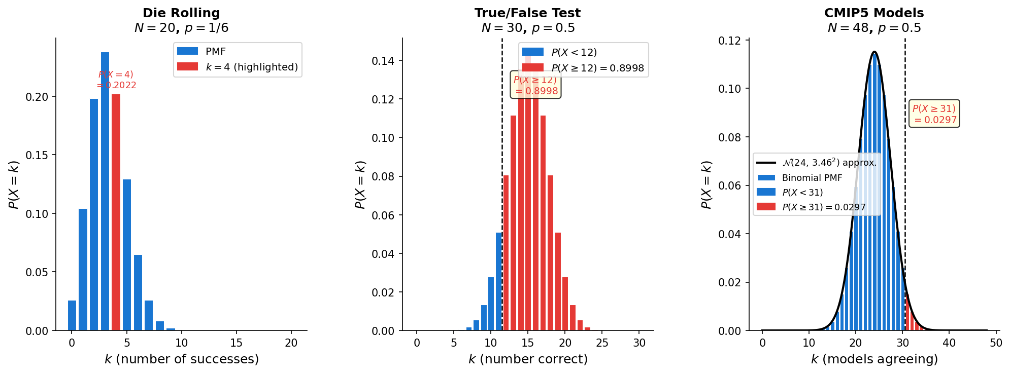
Normal Approximation to the Binomial#
You can probably imagine the problems getting much more tedious as you have to sum more and more. However, there is a normal approximation to the Binomial distribution in the case of
large \(N\)
\(Np > 10\)
\(N(1-p) > 10\)
In this case, the statistic
follows a Normal distribution with \(\mu = Np\) and \(\sigma = \sqrt{Np(1-p)}\).
An approximate two-tailed 95% confidence interval for the number of successes \(X\) is then,
Binomial Distribution I
What is the probability of rolling exactly 4 sixes out of 20 rolls of a fair 6-sided die?
Let’s define a success as rolling a six.
Binomial Distribution II
What is the probability of getting a score of 12 or more on a test of 30 true-false questions?
Let’s define a success as getting the question right.
Now, the problem is a bit more tedious, because we have to add up the probabilities for \(k = 12, 13, 14, \dots, 29, 30\). Instead, we can calculate the probability of getting \(k = 0, 1, 2, 3, \dots, 11\) questions right, and then 1 minus this probability is the probability we want. Thus,
Normal Approximation to the Binomial
48 CMIP5 models are discussed in the IPCC 5th Assessment Report. How many models must agree that global temperatures will increase by 2100 so that we can say with 95% certainty that the models do not agree purely by chance? What is the 95% confidence interval on the number of models with increasing temperatures under the null hypothesis?
Here, let a success be that the model says global temperatures will increase. Our null hypothesis is that the models randomly guess whether global temperatures will increase — thus, there is a 50% chance that any one model will predict a temperature increase (\(p=0.5\)). We want to know
Where \(k^*\) is the number of models required to show an increase in order for us to believe it is more than chance (that the null hypothesis can be rejected).
This would take a long time by hand, however, let’s check if the Normal approximation to the Binomial applies.
\(n\) is large (\(n=48\))
\(np = 24 > 10\)
\(n(1-p) = 24 > 10\)
So, we can use the Normal approximation for large \(N\):
So, at least 31 models are needed to predict increases — to reject the null hypothesis that it was due to random chance. As expected, more than half of the models must show an increase.
The 95% confidence interval under the null hypothesis is:
Non-parametric Tests#
Thus far, most of the statistics we have used assume an underlying distribution (typically normal). However, there may be instances where you do not think that the data is normally distributed — in which case, you might want to use a non-parametric statistical test.
Signs Test#
For example, say you want to test the null hypothesis that the means of two data sets \(x_i, y_i\) are identical. In this case, one could use the Signs Test, also known as the Wilcoxon Test.
Instead of testing the means, this test uses the medians (\(\tilde{\mu}\)) of the two distributions to determine if they are equal. We formulate the hypothesis in the following way.
To do this test, you replace each pair with a signed integer in the following manner:
The null hypothesis would suggest that there are a similar number of \(+1\) and \(-1\). With this setup, we now have a bunch of Bernoulli trials with a success (\(+1\)) and a failure (\(-1\)). Thus, we can use the Binomial Distribution to determine the probability of getting a certain number of \(+1\) versus \(-1\). Prof. Dennis Hartmann gives a nice example in Chapter 1.
Runs Test (Wald–Wolfowitz runs test)#
The runs test is a non-parametric test to check whether a data set is random or not. For example (taken from Wikipedia), imagine a time series on anomalies as shown below, where “+” denotes a positive anomaly and “\(-\)” denotes a negative anomaly:
+ + + + - - - + + + - - + + + + + + - - - -
We now separate this series into “runs”…specifically, there are \(R=6\) runs, 3 of which consist of “+” and the others of “\(-\)”. The runs test uses a null hypothesis that the data is random. Under this null hypothesis, the number of runs (\(R\)) in a sequence of \(N\) elements is a random variable whose conditional distribution given the observation of \(N_+\) positive values and \(N_-\) negative values (\(N = N_+ + N_-\)) has the following properties:
If \(N_+\) and \(N_-\) are sufficiently large (say, greater than 30) then the number of runs \(R\) is well modeled by a Normal distribution with parameters \(\mu\) and \(\sigma\) given above.
To test significance, standardize the observed number of runs \(R\) using
and compare \(z\) to the Normal distribution (or equivalently compare to critical values for your chosen \(\alpha\)).
Interpretation is intuitive:
Too few runs (\(R \ll \mu\)): neighboring values tend to have the same sign (persistence / clustering).
Too many runs (\(R \gg \mu\)): signs alternate more than expected (over-switching).
So the runs test is a simple way to ask whether your sequence behaves like random sign flips, or whether there is detectable serial structure.
Practical note for geophysical time series
For atmospheric and oceanic data, apparent significance can be affected by autocorrelation and by the threshold used to convert values into \(+\)/\(-\) signs. In practice, use the runs test as a quick diagnostic, then confirm conclusions with additional tools (e.g., autocorrelation analysis, block bootstrap, or Monte Carlo surrogates).
Summary and transition#
This chapter introduced the statistical foundations used throughout the rest of the course:
why the Gaussian emerges from an optimization principle,
how moments describe distributions,
how Bayes’ theorem updates belief with data,
how significance testing (z/t tests, confidence intervals, hypothesis tests) is applied,
and when resampling / non-parametric methods are preferable.
In the next part of the course, we build on these tools to analyze geophysical data where dependence, limited samples, and multiple-testing issues are the rule rather than the exception.