
Week 8-11: Seeking Structure in Data#
The pattern — Part III
This is the Part where the Lagrange multiplier of Chapter 0 stops being bookkeeping and becomes the answer:
The multiplier \(\lambda\) is the eigenvalue, which is the variance explained.
Clustering is the same move with a different functional — the within-cluster sum of squares — but its constraint needs care. “Exactly \(k\) clusters” is combinatorial, so it cannot carry a multiplier as written. Repair it one way and you recover this same equation, with the relaxed clustering turning out to be PCA (Part 6, Route 1); repair it the other way and the multiplier is a temperature that is the \(\beta\) of the variational autoencoder (Part 6 Route 2, and Part 7).
In Weeks 4-6 we asked a two-variable question: given \(x(t)\) and \(y(t)\), how strongly are they related? That question has an obvious limitation. A climate field is not two time series — it is thousands of grid points, each with its own time series, all correlated with one another in ways we would like to summarize.
This block is about finding structure in that kind of data: coherent spatial patterns that vary together in time, and groupings of observations that resemble one another. The two main tools are Empirical Orthogonal Function (EOF) analysis and cluster analysis.
The good news is that nothing here is conceptually new. EOF analysis is regression — the same projection of one vector onto another that gave us the correlation coefficient — applied simultaneously to every grid point, and organized so that the resulting patterns are uncorrelated with each other. What we need first is the language to write “every grid point at once” compactly, which is linear algebra.
Part 1 — Linear Algebra Review#
Matrix notation#
A matrix \(\mathbf{A}\) with \(M\) rows and \(N\) columns (dimensions \(M \times N\)) is ordered as
The notation \(a_{ij}\) denotes the element in the \(i\)th row and \(j\)th column, with \(1 \le i \le M\) and \(1 \le j \le N\).
A convention you must fix before you start
Almost every error in EOF analysis traces back to losing track of which dimension is space and which is time. Throughout these notes we will use
so \(M\) is the number of time steps and \(N\) is the number of grid points — except in the SVD section, where we follow Prof. Hartmann’s convention of space first. Every recipe below states its convention explicitly in the first line. Read it before you code.
Transpose#
The transpose of \(\mathbf{X}\) is written \(\mathbf{X}^T\) and is obtained by flipping rows and columns, so an \(M \times N\) matrix becomes \(N \times M\). In index notation, if \(\mathbf{X} = \mathbf{Y}^T\) then
Inner product — where regression re-enters#
All vectors are matrices whose second dimension is 1. If \(\mathbf{X}\) and \(\mathbf{Y}\) are two vectors of length \(M \times 1\), their inner product is
This is worth pausing on, because it is the bridge from Weeks 4-6:
if \(\mathbf{X}\) and \(\mathbf{Y}\) have mean zero, then \(\frac{1}{M}\mathbf{X}^T\mathbf{Y}\) is the covariance of the two vectors
if \(\mathbf{X}\) and \(\mathbf{Y}\) are additionally standardized (unit standard deviation), then \(\frac{1}{M}\mathbf{X}^T\mathbf{Y}\) is the correlation coefficient — and also the regression coefficient, since for standardized data \(a_1 = r\)
So an inner product is a regression. Everything in the EOF sections is built from this one operation.
Multiplying matrices#
If \(\mathbf{A}\) is \(M \times N\) and \(\mathbf{B}\) is \(N \times P\), then
The number of columns of the first matrix must equal the number of rows of the second. Unlike ordinary multiplication, matrix multiplication does not commute — you cannot re-order it.
To multiply, take the row of the first matrix against the column of the second, multiply element-wise and sum:
Covariance and correlation matrices#
This is the object the entire EOF machinery acts on. Given \(\mathbf{X}\) of dimension \(M \times N\) whose columns have mean zero,
is the covariance matrix, of dimension \(N \times N\). Element \(C_{ij}\) is the covariance between grid point \(i\) and grid point \(j\) — i.e. it is the inner product of column \(i\) with column \(j\), which by the previous section is exactly a covariance.
If the columns of \(\mathbf{X}\) are standardized rather than merely centered, the same expression
is the correlation matrix. The formula does not change; what changes is the preprocessing. This distinction returns in Part 3, because standardizing your data means you are eigenanalyzing the correlation matrix whether you intended to or not.
\(\mathbf{C}\) is also sometimes called the dispersion matrix. It is always square and always symmetric (\(\mathbf{C} = \mathbf{C}^T\)) — a fact we will lean on heavily.
Inverse#
The inverse of a square matrix \(\mathbf{X}\) is written \(\mathbf{X}^{-1}\). This does not mean raising the matrix to the \(-1\) power; it denotes the inverse specifically, defined by
where \(\mathbf{I}\) is the identity matrix — square, with ones on the diagonal and zeros elsewhere.
Only square matrices have inverses. (There are “left” and “right” inverses for non-square matrices, but we will not use them here.)
In ordinary algebra you divide to remove a multiplied variable. With matrices, you multiply by the inverse instead — that is what the inverse is for.
Types of matrices#
\(\mathbf{X}\) is diagonal if it is square with values along the diagonal and zeros everywhere else
\(\mathbf{X}\) is symmetric if \(\mathbf{X}^T = \mathbf{X}\)
\(\mathbf{X}\) is orthonormal if \(\mathbf{X}^T = \mathbf{X}^{-1}\), equivalently \(\mathbf{X}^T\mathbf{X} = \mathbf{X}\mathbf{X}^T = \mathbf{I}\)
That last one is the useful one. If all off-diagonal elements of \(\mathbf{X}^T\mathbf{X}\) are zero, then \(\mathbf{X}^T = \mathbf{X}^{-1}\), and all columns of \(\mathbf{X}\) are linearly independent — i.e. uncorrelated with one another. When we find that our EOFs form an orthonormal matrix, transposing will be all the “inverting” we ever need to do.
Vector spaces#
\(\mathbb{R}^0\): a single point (e.g. 0)
\(\mathbb{R}^1\): the real line
\(\mathbb{R}^2\): where all 2-element vectors live
\(\mathbb{R}^3\): 3-D space
Vector spaces are spanned by a set of basis vectors. A basis for \(\mathbb{R}^N\) is a set of \(N\) vectors that, through linear combination, can describe any vector in \(\mathbb{R}^N\).
There are infinitely many possible bases for any \(\mathbb{R}^N\), but the conventional choice is the unit vectors. For \(\mathbb{R}^2\):
Any point in \(\mathbb{R}^2\) is a linear combination of these — for example \((3,2) = 3\mathbf{e}_1 + 2\mathbf{e}_2\). Try it; you can reach anywhere in the plane.
Now a question. Do these form a basis for \(\mathbb{R}^2\)?
No — any point with a non-zero second component is unreachable. The direction \((0,1)\) and all its multiples form the null space: the part of the space these vectors cannot reach.
For \(\mathbb{R}^3\) the unit basis is
By definition basis vectors must be linearly independent — each supplies information the others do not.
Testing for a basis: determinants#
To check whether a set of vectors forms a basis, assemble them as the columns of \(\mathbf{A}\) and ask whether there is a non-trivial \(\mathbf{x}\) with
If such an \(\mathbf{x}\) exists, the vectors fail to span the space and/or are not all independent — there is a non-trivial null space.
Rather than solving for every \(\mathbf{x}\), we only need to know whether a solution exists, and there is a shortcut. If
then a non-trivial solution to \(\mathbf{A}\mathbf{x} = 0\) exists. Determinants are painful for large matrices but trivial for \(2\times2\):
If \(\mathbf{A}\) is square and \(\mathbf{A}\mathbf{x} = 0\) has a non-trivial solution, then \(\mathbf{A}\) is called singular or degenerate, and it has no inverse.
Rank#
The rank \(r\) of a matrix is the number of linearly independent columns. If \(\mathbf{A}\) holds the basis vectors of \(\mathbb{R}^2\),
so the rank is 2. But if
the columns are not independent. Here you can see it directly — twice the first column gives the second — but for larger matrices the determinant is what you rely on. The rank of this \(2\times2\) matrix is 1.
Rank is bounded by the smaller dimension:
If \(\mathbf{A}\) is \(N \times N\) and \(r < N\), there is a non-trivial null space; the directions in \(\mathbb{R}^N\) not spanned by the columns of \(\mathbf{A}\) define that null space.
columns linearly independent \(\Rightarrow\) \(\mathbf{A}\) is full rank
columns not linearly independent \(\Rightarrow\) \(\mathbf{A}\) is rank deficient
This matters practically: a rank-deficient covariance matrix has fewer non-zero eigenvalues than its dimension, which means fewer meaningful EOFs than grid points. If you have 100 time steps and 40000 grid points, your covariance matrix is \(40000\times40000\) but its rank is at most 100 — so at most 100 EOFs carry any information at all.
Part 2 — Eigenvalues and Eigenvectors#
Recall the covariance (dispersion) matrix
depending on which dimension is the sampling dimension. Either way \(\mathbf{C}\) is square and symmetric.
Principal Component Analysis is an eigenanalysis of \(\mathbf{C}\). Any symmetric matrix \(\mathbf{C}\) can be decomposed as
or in full matrix form
where \(\mathbf{E}\) has the eigenvectors \(\mathbf{e}_i\) as its columns, and \(\boldsymbol{\Lambda}\) is diagonal with the eigenvalues \(\lambda_i\) along it.
The set of eigenvectors and eigenvalues represents a coordinate transformation into a space where \(\mathbf{C}\) becomes diagonal. This is the whole idea, and it is worth stating carefully:
Because the covariance matrix is diagonal in this new coordinate space, the variations in these new directions are uncorrelated with each other. The eigenvectors define directions in the initial coordinate space along which the maximum possible variance can be explained, and in which variance in one direction is orthogonal to the variance explained by other directions defined by the other eigenvectors. The eigenvalues indicate how much variance is explained by each eigenvector.
— D. Hartmann notes, Chapter 4
Example / deeper dive
A worked \(2\times2\) eigenanalysis
Let the data be two points with the means already removed:
The covariance matrix is
and one can show that
Note that the norm of \(\mathbf{e}_1\) is 1. Check it against the eigenvalue equation:
so \(\lambda_1 = 2\). It turns out that \(\sum_i \lambda_i\) equals the total variance of \(\mathbf{A}\) — the sum of the diagonal of \(\mathbf{C}\), which here is 2. So in this problem there is only one non-zero eigenvalue (\(\lambda_2 = 0\)), and the first eigenvector explains all the variance.
That makes sense geometrically: both data points lie on the line \(y = -x\), so a single direction describes them completely.
Finally, note that
is an equally valid eigenvector. The overall sign of an eigenvector is arbitrary — which is why you should never over-interpret the sign of an EOF map without also looking at its PC.
Figure / in-class demonstration
Figure Example: eigenanalysis_2d.py — dots denote the points of \(\mathbf{A}\) with means removed, \((-1,1)\) and \((1,-1)\). Black coordinates denote the original \(x\)–\(y\) axes; purple coordinates denote positions along the new axis \(\mathbf{e}_1\), i.e. \((-\sqrt2, 0)\) and \((\sqrt2, 0)\). The two points and the dotted purple line (the direction of \(\mathbf{e}_1\)) lie along \(y = -x\).
A second panel adds a third point \((-1.1, -0.2)\) so the points no longer fall exactly on a line. Eigenanalysis now returns two eigenvectors \(\mathbf{e}_1\) and \(\mathbf{e}_2\), drawn as perpendicular dotted lines through the origin. Eigenvector 1 explains most of the variance; eigenvector 2 accounts for the deviations from it.
Solving for eigenvectors#
So the eigenvector \(\mathbf{e}_i\) lies in the null space of \((\mathbf{C} - \lambda_i\mathbf{I})\) — which is exactly the null-space machinery from Part 1. That matrix only has a null space if it is singular, i.e. if
Solving this is the eigenvalue problem, and it appears throughout science and engineering.
For a real, symmetric \(\mathbf{C}\) the eigenvalues \(\lambda_i\) are positive. If \(\mathbf{C}\) is \(M\times M\) there will be \(M\) eigenvalues and \(M\) eigenvectors — unless \(\mathbf{C}\) is degenerate, in which case there are only \(r\) of them, where \(r\) is the rank.
Properties of eigenvectors#
the eigenvectors of a matrix form a linearly independent set
if \(\mathbf{C}\) (\(M\times M\)) has full rank, the eigenvectors form a basis for \(\mathbb{R}^M\)
if \(\mathbf{C}\) is singular with rank \(r = k\), the first \(k\) eigenvectors span the subspace of \(\mathbf{C}\) (\(\mathbb{R}^k\)), and eigenvectors \(k+1 : M\) span the null space of \(\mathbf{C}\)
if \(\mathbf{C}\) is real and symmetric, the eigenvectors are not merely linearly independent, they are orthogonal
That last property is what puts the “O” in EOF, and we prove it in Part 3.
Terminology, precisely#
linearly independent: you cannot reach one vector by a linear combination of the others
orthogonal: the angle between the vectors is \(90^\circ\); they share no vector space
orthonormal: orthogonal and of unit length (\(\sqrt{x^2+y^2} = 1\))
Part 3 — EOFs via Eigenanalysis#
Figure / in-class demonstration
Show intro EOF slides: eofintro.pdf
A vocabulary note first, since the literature is loose about it:
EOF stands for Empirical Orthogonal Functions
PCA stands for Principal Component Analysis
the two are practically the same thing
PCA is the more general term, and just implies splitting a matrix into linearly uncorrelated variables called principal components
EOF analysis normally refers to finding the principal components that maximize variance explained — so, a subset of all the PCs
We will cover two routes to EOFs: eigenanalysis of the covariance matrix (this Part) and singular value decomposition (Part 4). Both give identical answers.
The picture to keep in your head#
Before any algebra, it is worth seeing what an EOF is geometrically. Everything below is a rotation of coordinate axes, and with only two grid points you can draw the whole thing on paper.
Example / deeper dive
EOFs are the axes of the scatter cloud
Take two stations, \(N = 2\), so every observation is a point in a plane: \(x\) is the anomaly at station A, \(y\) the anomaly at station B. Eight observation times, \(M = 8\):
Both columns already sum to zero, so this is an anomaly matrix. Plotted as dots, the data form a tilted, cigar-shaped cloud:
Run eof_scatter_2d.py to generate this figure.
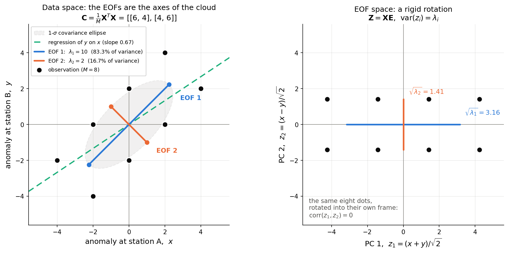
The script runs the full recipe in nine lines of numpy — form \(\mathbf{C}\), call numpy.linalg.eigh, sort the eigenvalues descending, project — and prints the numbers derived by hand below. The left panel is the cloud in data space with the EOF axes drawn; the right panel is the same eight dots after the rotation \(\mathbf{Z} = \mathbf{XE}\).
The covariance matrix. With \(M = 8\),
The eigenanalysis. For a matrix of the form \(\begin{bmatrix}a & b\\ b & a\end{bmatrix}\) the eigenvalues are \(a \pm b\):
Check: \(\mathbf{C}\mathbf{e}_1 = \tfrac{1}{\sqrt2}(10,10)^T = 10\,\mathbf{e}_1\), \(\mathbf{e}_1^T\mathbf{e}_2 = 0\), and \(\lambda_1 + \lambda_2 = 12 = \mathrm{tr}(\mathbf{C})\). EOF 1 explains \(10/12 = 83.3\%\) of the variance, EOF 2 the remaining \(16.7\%\).
The PCs are simply the coordinates of each dot measured along the new axes, \(\mathbf{Z} = \mathbf{X}\mathbf{E}\):
with \(\mathrm{var}(\mathbf{z}_1) = 10 = \lambda_1\), \(\mathrm{var}(\mathbf{z}_2) = 2 = \lambda_2\), and \(\mathbf{z}_1^T\mathbf{z}_2 = 0\) — the PCs are uncorrelated, which is the entire point of diagonalizing \(\mathbf{C}\).
The dictionary between the algebra and the picture:
Algebra |
Geometry |
|---|---|
\(\mathbf{e}_1\) |
direction of the major axis of the scatter ellipse |
\(\mathbf{e}_2\) |
minor axis, forced perpendicular to \(\mathbf{e}_1\) |
\(\sqrt{\lambda_i}\) |
half-length of the ellipse along axis \(i\); here \(\sqrt{10}:\sqrt{2} = \sqrt5 \approx 2.24\), so the cloud is 2.24 times longer than it is wide |
\(z_i(t)\) |
the coordinate of dot \(t\) along axis \(i\) |
the whole analysis |
a rigid rotation of the axes into the cloud’s own frame |
The tilt angle in general is \(\tan 2\theta = 2c_{xy}/(c_{xx} - c_{yy})\). Here the denominator vanishes, so \(\theta = 45^\circ\) exactly: whenever two variables have equal variance, EOF 1 bisects them no matter how strong the correlation. The correlation (\(r = 4/6 = 0.67\)) sets the ellipse’s eccentricity, not its orientation.
Three things the picture makes obvious:
EOF 1 is not the regression line. Regressing \(y\) on \(x\) gives slope \(c_{xy}/c_{xx} = 2/3\), not 1. Regression minimizes vertical distance to the line; EOF 1 minimizes perpendicular distance. The two coincide only when \(r = \pm1\).
The sign is arbitrary. \(-\mathbf{e}_1\) is an equally valid axis — an axis has a direction, not an arrowhead. Flipping \(\mathbf{e}_1\) flips \(\mathbf{z}_1\) and leaves the product \(\mathbf{z}_1\mathbf{e}_1^T\) untouched.
Orthogonality is imposed, not discovered. EOF 2 had no freedom at all: in two dimensions, once EOF 1 is fixed there is only one unit direction left. That is the geometric root of the warning in Part 5 — higher EOFs are shaped as much by the EOFs before them as by the physics.
Physically, \(\mathbf{e}_1 = (1,1)/\sqrt2\) is the two stations warming together and \(\mathbf{e}_2 = (1,-1)/\sqrt2\) is a seesaw between them — the same uniform-versus-dipole story as the four-point basin worked through at the end of this Part, but small enough to draw.
Setting up the maximization#
Let \(\mathbf{X}\) be \(M \times N\), rows being times and columns being spatial locations. We want to decompose \(\mathbf{X}\) into orthogonal eigenvectors that explain the most variance. Equivalently, we want to find the \(\mathbf{e}_1\) (dimension \([N\times1]\), i.e. a spatial pattern) that most resembles the data.
Building the measure of “resemblance”, one requirement at a time:
the projection of \(\mathbf{e}_1\) onto the data is measured by the inner product of \(\mathbf{e}_1\) with \(\mathbf{X}\) — this is the resemblance
the projection is squared, so that positive and negative resemblance count the same (exactly as in linear regression, where we squared the errors)
to make the measure independent of the number of observations, divide by \(M\)
to make it independent of the magnitude of \(\mathbf{e}_1\), normalize to unit length, \(\mathbf{e}_1^T\mathbf{e}_1 = 1\) — otherwise the projection could be made arbitrarily large just by lengthening \(\mathbf{e}_1\)
following these rules, the measure of resemblance is
which is equivalent to maximizing
Call the maximum value of this squared projection \(\lambda_1\) — the variance explained by \(\mathbf{e}_1\):
This has exactly the form of the eigenvalue problem from Part 2. Since the norm of \(\mathbf{e}_1\) is one, it becomes
and in full matrix notation (with \(\mathbf{C}\), \(\boldsymbol{\Lambda}\), \(\mathbf{E}\) all \(N \times N\)),
using \(\mathbf{E}^T\mathbf{E} = \mathbf{E}\mathbf{E}^T = \mathbf{I}\).
So \(\mathbf{e}_1\) must be an eigenvector of \(\mathbf{C}\). We find it by eigenanalyzing \(\mathbf{C}\) and taking the eigenvector belonging to the largest eigenvalue. The search for “the pattern that explains the most variance” and the eigenvalue problem are the same problem.
What this buys you#
the 1st eigenvector explains the most variance in \(\mathbf{X}\) and has the largest eigenvalue
the 2nd eigenvector explains the second most, with the 2nd largest eigenvalue
the eigenanalysis transforms \(\mathbf{C}\) into a coordinate system where the new dispersion matrix is diagonal (\(\boldsymbol{\Lambda}\))
in that space all the variance is on the diagonal, since the vectors are orthogonal, so the fraction of variance explained by the \(j\)th eigenvector is
EOFs are conventionally ordered by \(\lambda\), so EOF 1 explains the largest variance and the last EOF the smallest
no other linear combination of \(k\) predictors can explain a larger fraction of the variance than the first \(k\) EOF/PC pairs
That final point is the reason EOFs are used for compression and noise reduction: they are optimal in the variance sense, by construction.
Example / deeper dive
Proof that eigenvectors are orthogonal
Suppose we have two eigenvectors \(\mathbf{e}_j\) and \(\mathbf{e}_k\):
Multiply the \(j\)th equation by \(\mathbf{e}_k^T\) and take the transpose; multiply the \(k\)th by \(\mathbf{e}_j^T\); subtract. This gives
Since \(\mathbf{C}\) is symmetric, \(\mathbf{C} = \mathbf{C}^T\), so the left-hand side vanishes. Therefore
The eigenvectors are orthogonal provided the eigenvalues are distinct. Hold onto that caveat — it comes back in Part 5, where eigenvalues that are not well separated turn out to be the central practical problem in EOF analysis.
Getting your original data back#
We want to keep all the original information in the new coordinate system, so we need the amplitudes that express each state in the EOF basis. Define
Then, since \(\mathbf{E}\mathbf{E}^T = \mathbf{I}\),
The columns of \(\mathbf{Z}\) are the principal components (PCs), of length \(M\). They tell you how much a given sample resembles a particular EOF structure.
To reconstruct a single observation at time \(t\) and location \(i\), combine the eigenvectors linearly with the PC amplitudes:
Concretely, suppose the first eigenvector is
Project it onto the original data to get its amplitude at each time step:
that is, \(\mathbf{X}\mathbf{E} = \mathbf{Z}\).
A common mistake
Project \(\mathbf{e}\) onto the original data \(\mathbf{X}\), not onto the covariance matrix \(\mathbf{C}\). The covariance matrix has already had the time dimension summed out of it — there is no time series left in it to recover.
Practical considerations: which covariance matrix?#
The covariance matrix can be formed two ways:
So far we have used the first. Which you should use is purely a question of computational cost:
\(M = 20000\) days, \(N = 400\) grid points \(\Rightarrow\) use \(\frac{1}{M}\mathbf{X}^T\mathbf{X}\), a \(400\times400\) problem. Easy.
\(M = 100\) days, \(N = 40000\) grid points \(\Rightarrow\) \(\frac{1}{M}\mathbf{X}^T\mathbf{X}\) would be \(40000\times40000\). Not easy.
In the second case you have two options:
interpolate your data onto a coarser mesh
perform the eigenanalysis on the spatial dispersion matrix, \(\mathbf{C} = \frac{1}{N}\mathbf{X}\mathbf{X}^T\), which is only \(100\times100\)
Option 2 gives the same answer, with one twist you must remember: the eigenvectors are now the PCs, and the PCs are now the EOFs. The roles swap. Recall from Part 1 that the rank of that giant \(40000\times40000\) matrix was at most 100 anyway — so nothing is lost by working in the smaller space.
Summary: EOFs by eigenanalysis of the covariance matrix, \(\mathbf{X} = [M\times N]\)#
subtract the mean along the sampling dimension of \(\mathbf{X}\)
unless data size forces otherwise, define \(\mathbf{C}\) along the sampling dimension so you are left with the space dimension:
eigenanalyze \(\mathbf{C}\) by diagonalizing it (
eigin Matlab,EIGENQLin IDL,numpy.linalg.eighin Python)the first EOF is the eigenvector corresponding to the largest eigenvalue
to find the PCs, project the data onto the eigenvectors — PCs should have the length of your sampling dimension
the fraction of variance explained by the \(i\)th EOF pair is \(\lambda_i/\sum_j\lambda_j\)
Example / deeper dive
A complete EOF analysis you can do by hand
The \(2\times2\) example in Part 2 showed the eigenanalysis. This one runs the whole recipe end to end, on numbers small enough to check with a pencil.
The data. Imagine a basin with four grid points in a row, observed at four times. The anomaly matrix \(\mathbf{X} = [M\times N] = [4 \text{ times} \times 4 \text{ points}]\) is
Reading the rows: at time 1 the west half is warm and the east half is cool; at time 2 it has flipped. There is a seesaw in the data, plus something weaker going on.
Step 1 — remove the sampling mean. Each column already sums to zero, so \(\mathbf{X}\) is already an anomaly matrix. (Check: \(3-1+1-3 = 0\).)
Step 2 — form the covariance matrix. With \(M = 4\),
It is square, symmetric, and \(4\times4\) because we contracted over time. Points 1 and 2 covary positively (\(+5\)); points 1 and 3 covary negatively (\(-3\)). The total variance is \(\mathrm{tr}(\mathbf{C}) = 20\).
Step 3 — eigenanalyze. Two eigenvalues are non-zero:
Verify the first one directly: \(\mathbf{C}\mathbf{e}_1 = (8,8,-8,-8)^T = 16\,\mathbf{e}_1\). Both vectors have unit norm (\(4\times(\tfrac12)^2 = 1\)) and are orthogonal (\(\mathbf{e}_1^T\mathbf{e}_2 = 0\)), as Part 3 promised they must be. Note also \(\sum_i\lambda_i = 16+4 = 20 = \mathrm{tr}(\mathbf{C})\): the eigenvalues redistribute the total variance, they do not create or destroy it.
Step 4 — EOF 1. The leading eigenvector is the dipole \((+,+,-,-)\): the west-versus-east seesaw. EOF 2 is the uniform pattern \((+,+,+,+)\): the whole basin warming or cooling together.
Step 5 — the PCs. Project the data onto the eigenvectors, \(\mathbf{Z} = \mathbf{X}\mathbf{E}\):
Each has length \(M = 4\), as it must. PC 1 flips sign every time step — the seesaw oscillating fast. PC 2 switches sign once, halfway through — a slow basin-wide drift. And \(\mathbf{z}_1^T\mathbf{z}_2 = 0\): the PCs are uncorrelated, which is the whole point of diagonalizing \(\mathbf{C}\). Note too that \(\mathrm{var}(\mathbf{z}_1) = 16 = \lambda_1\) — the eigenvalue is the variance of its PC.
Step 6 — variance explained.
Two EOFs account for everything. That is not luck: we built \(\mathbf{X}\) from exactly two patterns, so its rank is 2, and by the rank argument in Part 1 a rank-2 matrix cannot have more than two non-zero eigenvalues. The \(4\times4\) covariance matrix is degenerate, and \(\mathbf{e}_3,\mathbf{e}_4\) span its null space. Whatever your eigensolver returns for them is numerical noise — a situation you meet constantly with real data, where \(N\) grid points vastly outnumber \(M\) time steps.
Putting it back together. Because the decomposition is complete,
Check row 1: \(4\cdot(\tfrac12,\tfrac12,-\tfrac12,-\tfrac12) + 2\cdot(\tfrac12,\tfrac12,\tfrac12,\tfrac12) = (2,2,-2,-2)+(1,1,1,1) = (3,3,-1,-1)\). ✓
Physical units (looking ahead to Part 5). \(\mathbf{e}_1\) has no units — its entries are \(\pm\tfrac12\) because we forced unit norm. Standardize PC 1 (its mean is already zero, and \(\sigma_{z_1} = 4\)) to get \(\tilde{\mathbf{z}}_1 = (1,-1,1,-1)^T\), then regress it back onto the data:
This is a sentence you can defend in a caption: a one-standard-deviation swing of PC 1 corresponds to a \(+2\) anomaly at the two western points and \(-2\) at the two eastern points. Observe that \(\mathbf{d}_1 = \sigma_{z_1}\mathbf{e}_1\) exactly — because here we neither area-weighted nor standardized, the pattern is unchanged and only the scaling differs, precisely as noted in Recipe 1 step 8.
One caution. EOF 1 came out as the dipole because the dipole carried the most variance, not because it is more “physical” than the uniform mode. Had we multiplied the uniform pattern’s amplitude by 3, EOF 1 would be the uniform mode instead, with the dipole demoted to EOF 2. The ordering is a statement about variance, nothing more — a point that returns with force in Part 5.
Figure / in-class demonstration
Show slides: eof_physicalvars.pdf
Show webpage: Eigenstyle — http://blog.thehackerati.com/post/126701202241/eigenstyle (PCA applied to a wardrobe of dresses; a memorable demonstration that “EOF 1” is just “the direction of greatest variance”, whatever the data happen to be).
Part 4 — EOFs via Singular Value Decomposition (SVD)#
There is a second route to the same answer, and in practice it is the one you will use. SVD is more general, more numerically stable, and skips the explicit formation of \(\mathbf{C}\) entirely.
Any \(M\times N\) matrix can be decomposed into a product of three matrices:
where
\(\mathbf{U}\) is \(M\times M\)
\(\boldsymbol{\Sigma}\) is \(M\times N\)
\(\mathbf{V}\) is \(N\times N\)
\(\mathbf{U}\) and \(\mathbf{V}\) are orthogonal
\(\boldsymbol{\Sigma}\) is diagonal
If we let the \(M\) dimension be space and the \(N\) dimension be time (following Prof. Hartmann’s notes — note this is the opposite of Part 3), then:
the columns of \(\mathbf{U}\) are the eigenvectors of \(\mathbf{X}\mathbf{X}^T\) — the EOFs
the columns of \(\mathbf{V}\) (rows of \(\mathbf{V}^T\)) are the eigenvectors of \(\mathbf{X}^T\mathbf{X}\) — the PCs
the \(r\) singular values along the diagonal of \(\boldsymbol{\Sigma}\) are proportional to the square roots of the non-zero eigenvalues of both \(\mathbf{X}\mathbf{X}^T\) and \(\mathbf{X}^T\mathbf{X}\): \(s_i = \sqrt{\lambda_i}\)
to get variance explained, square the elements of \(\boldsymbol{\Sigma}\)
Watch your dimension order
If instead you have time along \(M\) and space along \(N\) (the Part 3 convention), then the columns of \(\mathbf{V}\) are the EOFs and the columns of \(\mathbf{U}\) are the PCs. Everything else is identical. The mathematics does not care; you do.
The matrix \(\boldsymbol{\Sigma}\) is odd in that it is not square, yet we care about its diagonal. It can be viewed two ways:
if \(M > N\),
where \(\mathbf{D}\) is \(N\times N\) diagonal and \(\mathbf{0}\) is \((M-N)\times N\) zeros. The first \(r\) elements of \(\mathbf{D}\) are the singular values.
if \(\mathbf{X}\) is full rank and \(M = N\), then \(\boldsymbol{\Sigma}\) is genuinely square and diagonal.
If the singular values are ordered with \(\sigma_1\) largest, then the first column of \(\mathbf{U}\) is the leading EOF and the first column of \(\mathbf{V}\) is the leading PC.
Example / deeper dive
Why SVD and eigenanalysis give the same EOFs
Start from the SVD of \(\mathbf{X}\) and square both sides:
Since \(\mathbf{V}^T\mathbf{V} = \mathbf{I}\) (the columns of \(\mathbf{U}\) and \(\mathbf{V}\) are made orthonormal),
Multiplying both sides by \(\mathbf{U}\),
Compare with the eigenanalysis of the covariance matrix, \(\mathbf{C}\mathbf{U} = \mathbf{U}\boldsymbol{\Lambda}\). Therefore
and \(\mathbf{U}\) holds the eigenvectors of \(\mathbf{C}\). The two methods are the same calculation.
Similarly for the PCs: starting again from \(\mathbf{X} = \mathbf{U}\boldsymbol{\Sigma}\mathbf{V}^T\) and writing \(\mathbf{X} = \mathbf{U}\mathbf{Z}\), we identify
which is consistent with \(\mathbf{X} = \mathbf{E}\mathbf{Z}\) from the eigenanalysis, since \(\mathbf{U} = \mathbf{E}\).
Numerical check. Take the \(4\times4\) matrix \(\mathbf{X}\) from the worked example in Part 3 and hand it to an SVD routine. The singular values come back as
That matrix is \([\text{time}\times\text{space}]\) — the Part 3 convention — so by the warning box above the EOFs are the columns of \(\mathbf{V}\), and indeed \(\mathbf{V}\)’s first column is \(\pm\tfrac12(1,1,-1,-1)^T\): the same dipole, possibly with the sign flipped, which as always carries no meaning. The variance fractions agree too,
and \(s_i^2/M = (16, 4, 0, 0)\) recovers the eigenvalues of \(\mathbf{C}\) exactly, which is the relation \(\frac{1}{M}\boldsymbol{\Sigma}^2 = \boldsymbol{\Lambda}\) just derived. Two zero singular values, again flagging rank 2.
Summary: EOFs with SVD, \(\mathbf{X} = [M\times N]\)#
subtract the mean along the sampling dimension of \(\mathbf{X}\)
decompose \(\mathbf{X}\) with a built-in SVD routine
if \(M\) is the sample dimension (time), the EOFs (spatial patterns) are the columns of \(\mathbf{V}\) and the PCs (time series) the columns of \(\mathbf{U}\)
if \(N\) is the sample dimension (time), the EOFs are \(\mathbf{U}\) and the PCs are \(\mathbf{V}\)
the fraction of variance explained by the \(i\)th EOF pair is \(\sigma_i^2/\sum_j\sigma_j^2\)
Part 5 — EOFs with Actual Data#
The mathematics above is exact. Applying it to real geophysical data introduces a set of choices that the mathematics will not make for you, and which change your answer.
Preparing the data#
Removing the sampling mean
it is standard to remove the mean along the sampling dimension
this makes your PCs have zero mean
you may also want to remove the seasonal cycle (or diurnal cycle) if it is not of interest — otherwise EOF 1 will simply be the seasonal cycle, which you already knew about
Removing the spatial mean
less common, since you usually want to allow EOFs to have the same sign everywhere
exceptions: you care about temperature gradients rather than the full field
or you care about the eddy component, so you remove the zonal mean
Standardizing the data
Sometimes you want to remove amplitude information before the analysis:
your data combine parameters with different units, and you don’t want the one with the largest units to dominate the variance
the variance varies greatly from place to place and that variation is not of interest
To do this, after subtracting the sampling-dimension mean, divide by the standard deviation — your data are now in units of \(\sigma\). Note the consequence flagged back in Part 1: you are now eigenanalyzing the correlation matrix, not the covariance matrix.
Weighting
Gridded data must be weighted by grid area, or high-latitude grid points — which represent much less area — will be over-represented:
temporal covariance matrix: weight by \(\sqrt{\cos\theta}\) (when grid points are multiplied against each other in forming \(\mathbf{C}\), you recover the full \(\cos\theta\))
spatial dispersion matrix: weight by \(\cos\theta\), but carefully — \(\mathbf{C} = \mathbf{X}_{\cos}^T\mathbf{X}_{\cos}\) where the elements of \(\mathbf{X}_{\cos}\) are \(x_{t,\theta}\times\cos(\theta)\)
SVD: weight your data by \(\cos\theta\)
The resulting EOF will look unphysical and carry unphysical values. That is expected, and is fixed at the presentation stage below.
Missing data
most routines will not perform eigenanalysis or SVD with NaNs present
the best option is to use only locations with at least \(\alpha\%\) of data present, and to compute EOFs via the covariance matrix so that \(\mathbf{C}\) contains no missing values when passed to the eigenanalysis routine
Presentation of EOFs#
Let \(\mathbf{X}\) be \([M\times N]\) with \(M\) samples and \(N\) locations. From here on we write equations for EOF 1 and PC 1 only; repeat for the others.
Both EOFs and PCs get plotted in the literature depending on interest. Generally the spatial domain is the more interesting one, since the PC time series is usually noisy.
Problem: the EOFs have no physical units, so we need a meaningful way to plot the patterns.
The procedure:
calculate the leading PC \(\mathbf{z}_1\) (directly from SVD, or by projection in the eigenanalysis method)
standardize \(\mathbf{z}_1\) — the mean is already zero, so just divide by \(\sigma_{z_1}\)
project the standardized PC back onto your original anomaly data and divide by the length of \(\mathbf{z}\), giving \(\mathbf{d}_1\): EOF 1 in the units of the original, unweighted data
If the original data is \(\mathbf{X}\) and the weighted data is \(\mathbf{X}_w\), then following eigenanalysis:
Now \(\mathbf{d}_1\) is in physical units, and means: the anomaly associated with a one-standard-deviation variation of \(\mathbf{z}_1\). That is a statement you can put in a figure caption and defend.
Note this works for both the covariance method and SVD. For SVD there is one fewer step, since the raw PC 1 is handed to you.
Note also that this last step is a regression — projecting a standardized time series onto data, exactly as in Weeks 4-6. The EOF gave us the pattern; regression gives it units.
How many EOFs should be retained?#
This is the question that separates careful EOF analysis from decorative EOF analysis.
EOFs will always give you an answer. EOFs of red noise will produce sines and cosines that look thoroughly physical. The rate at which eigenvalues drop off is a function of the redness of the data, not of whether anything meaningful is present.
Worse, orthogonality itself imposes a constraint on shape. Higher-order EOFs are often trying to represent noise while remaining orthogonal to everything before them — so their structure is partly an artifact of the EOFs that preceded them, not of the physics.
North et al. (1982) argue that the significance of an EOF is a function of how well separated the eigenvalues are. The 95% confidence bounds on an eigenvalue are
Here \(N^*\) is our friend the effective degrees of freedom from Weeks 4-6 — autocorrelated data has fewer independent samples than it has data points. This is not easy to compute, and note you need a single value representative of the entire data set.
If the confidence bounds of two eigenvalues overlap, those two EOFs are effectively degenerate: they cannot be distinguished, and their individual patterns should not be interpreted. This is the practical face of the caveat from the orthogonality proof in Part 3 — the eigenvectors are only orthogonal (and only uniquely determined) if the eigenvalues are distinct.
When in doubt, test robustness other ways:
subdivide your sample and compare EOF structures — are they the same?
are your results explainable through theory?
are results sensitive to the size of the domain? (high sensitivity suggests you are fitting sines and cosines inside your boundaries)
Figure / in-class demonstration
Figure: Eigenvalue spectrum with North et al. (1982) bounds — variance explained (%) on the \(y\)-axis (0–20%) against eigenvalue index (1–25), with error bars showing the 95% confidence bounds. Two series: an orange “random sample” curve decaying gradually and smoothly from about 15% to under 5%, and a purple “sample with structure” curve starting near 20% at index 1, dropping sharply to about 7% by index 2, then decaying like the random sample — illustrating a single dominant, well-separated leading EOF.
Wave-like phenomena. If a travelling wave is present in your data, it appears as two eigenvalues close together and separated from the rest. These are the paired sine and cosine components of the wave. Do not interpret them as two independent patterns; they are one propagating feature.
Figure / in-class demonstration
Matlab examples: EOF_from_scratch.m, EOF_smoothing.m, eof_noise_reduction.m
Recipe 1: EOFs from the temporal covariance matrix#
Assume \(\mathbf{X} = [M\times N] = [\text{sampling}\times\text{space}]\); \(\mathbf{e}_1, \mathbf{d}_1 = [N\times1]\) and \(\mathbf{z}_1 = [M\times1]\).
1. Prepare the data
calculate anomalies along the sampling dimension, call this \(\mathbf{X}\) — may be just the sample mean, or may include removing the seasonal cycle
decide whether to standardize (divide by the standard deviation along the sampling dimension) — call this \(\mathbf{X}_w\)
save your original anomaly matrix \(\mathbf{X}\) — you will need it in step 8
2. Calculate the temporal covariance matrix
\(\mathbf{C} = \frac{1}{M}\mathbf{X}_w^T\mathbf{X}_w\)
if area weighting is needed, multiply \(\mathbf{X}\) by \(\sqrt{\cos\theta}\) first (call it \(\mathbf{X}_w\)), then form \(\mathbf{C}\)
3. Perform eigenanalysis
use a built-in routine; it returns eigenvectors \(\mathbf{E}\) and eigenvalues \(\boldsymbol{\Lambda}\)
[E, Lambda] = eig(C);in Matlab
4. Calculate and plot variance explained
\(\lambda_i/\sum_j\lambda_j\)
plot it and determine which of the first few are distinct — use the North et al. (1982) bounds \(\Delta\lambda = \lambda\sqrt{2/N^*}\) and look for non-overlap
5. Retain the EOFs you are interested in
keep those with interesting variance explained; this may be only the first column of \(\mathbf{E}\), denoted \(\mathbf{e}_1\)
6. Calculate the PCs
project the weighted/standardized anomaly matrix onto the eigenvectors: \(\mathbf{z}_1 = \mathbf{X}_w\mathbf{e}_1\), \(\mathbf{z}_2 = \mathbf{X}_w\mathbf{e}_2\), …
7. Standardize the PCs
\(\tilde{\mathbf{z}}_1 = (\mathbf{z}_1 - \mu_{z_1})/\sigma_{z_1}\)
\(\tilde{\mathbf{z}}_1\) is now in units of \(\sigma\) — this is the PC to use from here on
8. Calculate EOFs in physical units
\(\mathbf{d}_1 = \frac{1}{M}\tilde{\mathbf{z}}_1^T\mathbf{X}\), projecting onto the original anomaly data
\(\mathbf{d}_1\) is in the units of your data: the anomaly associated with a one-\(\sigma\) variation of the PC
if \(\mathbf{X} \equiv \mathbf{X}_w\), then \(\mathbf{d}_1\) has the same pattern as \(\mathbf{e}_1\) with different values; but if you area-weighted or standardized, the spatial patterns will genuinely differ
Recipe 2: EOFs from the spatial dispersion matrix#
Same dimensions as Recipe 1. Use this when \(N \gg M\).
1. Prepare the data — as in Recipe 1.
2. Calculate the spatial dispersion matrix
\(\mathbf{C} = \frac{1}{N}\mathbf{X}_w\mathbf{X}_w^T\)
for area weighting, let \(\mathbf{X}_{w,\cos}\) be the elements of \(\mathbf{X}_w\) multiplied by \(\cos\theta\), then \(\mathbf{C} = \frac{1}{N}\mathbf{X}_{w,\cos}\mathbf{X}_w^T\)
3. Perform eigenanalysis
the routine now returns your PCs in \(\mathbf{E}\) and eigenvalues in \(\boldsymbol{\Lambda}\) — the roles have swapped
4. Calculate and plot variance explained — as in Recipe 1.
5. Retain the PCs you are interested in
keep the first column of \(\mathbf{E}\), denoted \(\mathbf{z}_1\) — this is actually the first PC, because you analyzed the dispersion matrix
6. Standardize the PCs
\(\tilde{\mathbf{z}}_1 = (\mathbf{z}_1 - \mu_{z_1})/\sigma_{z_1}\)
7. Calculate EOFs in physical units
\(\mathbf{d}_1 = \frac{1}{M}\tilde{\mathbf{z}}_1^T\mathbf{X}\), \(\mathbf{d}_2 = \frac{1}{M}\tilde{\mathbf{z}}_2^T\mathbf{X}\), …
again in the units of the original data
Note that this recipe has one step fewer than Recipe 1: you never have to project to get the PCs, because the eigenanalysis handed them to you directly.
Recipe 3: EOFs via SVD#
Assume \(\mathbf{X} = [N\times M] = [\text{space}\times\text{sampling}]\); \(\mathbf{e}_1, \mathbf{d}_1 = [N\times1]\); \(\mathbf{z}_1 = [M\times1]\). Note the transposed convention.
1. Prepare the data
calculate anomalies along the sampling dimension
decide whether to standardize — call it \(\mathbf{X}_w\)
if area weighting is needed, weight \(\mathbf{X}\) by \(\cos(\text{latitude})\) and call it \(\mathbf{X}_w\)
save the original anomaly matrix \(\mathbf{X}\)
2. Perform SVD
[U, Sigma, V] = svd(Xw);in Matlabthe eigenvectors are the columns of \(\mathbf{U}\), the PCs the columns of \(\mathbf{V}\), the singular values the diagonal of \(\boldsymbol{\Sigma}\)
3. Calculate and plot variance explained
\(s_i^2/\sum_j s_j^2\) — note the square, since singular values are square roots of eigenvalues
apply the North et al. bounds as before
4. Retain the EOFs you are interested in
the first column of \(\mathbf{U}\), denoted \(\mathbf{e}_1\)
5. Calculate PCs
already done for you: PC 1 is the first column of \(\mathbf{V}\), denoted \(\mathbf{z}_1\)
6. Standardize the PCs
\(\tilde{\mathbf{z}}_1 = (\mathbf{z}_1 - \mu_{z_1})/\sigma_{z_1}\)
7. Calculate EOFs in physical units
\(\mathbf{d}_1 = \frac{1}{M}\mathbf{X}\tilde{\mathbf{z}}_1\), \(\mathbf{d}_2 = \frac{1}{M}\mathbf{X}\tilde{\mathbf{z}}_2\), …
note the ordering differs from Recipes 1–2 because of the transposed convention
as before, if you weighted or standardized, the pattern of \(\mathbf{d}_1\) will genuinely differ from \(\mathbf{e}_1\)
Part 6 — Cluster Analysis#
Cluster analysis is a data-mining technique whose goal is to group observations into a number of distinct clusters. Each observation ends up in exactly one cluster, with the assignment determined by a cost function. Finding the optimal set of clusters is usually iterative, starting from an initial guess.
The contrast with EOF analysis is the important part. Recall that a principal component tells you how much a given observation resembles a particular EOF pattern. An observation may look predominantly like one EOF — a large PC for that mode — but it will still have non-zero PCs for all the others. Every observation is a mixture of all the patterns.
In cluster analysis this is not so: each observation belongs to one cluster and no other. EOFs decompose; clusters partition. Which you want depends on whether you believe your system moves continuously through a state space or occupies discrete preferred regimes.
k-means clustering#
k-means is the most popular clustering technique in Earth science, largely for its simplicity. The aim is to group the \(M\) observations into \(k\) clusters, each observation belonging to the cluster with the nearest center. This partitions the data into Voronoi cells.
Which dimension gets partitioned
Keep the Part 1 convention in view: \(\mathbf{X} = [M\times N] = [\text{sampling}\times\text{space}]\). Cluster analysis groups samples, so what gets partitioned is the \(M\) rows — each row one observation, i.e. one point in the \(N\)-dimensional space of grid points. EOF analysis contracted over \(M\) to find structure in \(N\); clustering keeps all \(N\) coordinates and groups in \(M\). Same matrix, opposite dimension.
The optimal distribution of cluster centers minimizes the within-cluster sum of squares — the sum of distances from each point to its cluster center:
where \(S = \{S_1, S_2, \ldots, S_k\}\) is the set of \(k\) clusters, \(\mathbf{x}\) the observations, \(\boldsymbol{\mu}_i\) the center of cluster \(S_i\) (the mean of all points in it), and \(\arg\min\) indicates we seek the minimum over possible partitions \(S\).
Note that this is a sum of squared distances — the same least-squares logic as linear regression in Weeks 4-6 and the same squared projection that defined EOF 1 in Part 3. Squaring keeps the cost positive definite and makes the minimization tractable, at the price of weighting outliers heavily.
What k-means actually optimizes#
The opening admonition of this Part promised that k-means is the Chapter 0 move with a different functional and a different constraint. It is time to pay that off, because doing so turns out to connect k-means directly to the EOFs of Part 3 and to the \(\beta\) of Part 7.
First, the centroid update is not a choice. Hold the assignment \(S\) fixed and differentiate \(J\) with respect to one center:
So step (ii) of Lloyd’s algorithm — “recompute each center as the mean of its points” — is not a sensible-looking heuristic; it is the stationary condition of the cost function. Step (i), reassigning each point to its nearest center, is the exact minimization over \(S\) with \(\boldsymbol\mu\) held fixed. Lloyd’s algorithm is coordinate descent: alternate exact minimization over two blocks of variables. Each half-step can only decrease \(J\), and \(J\ge0\), so it must converge — but it converges to a point where neither block can improve alone, which is precisely why the optimum is local and why you run it many times.
Where is the Lagrange multiplier?
Chapter 0’s table lists the clustering constraint as “exactly \(k\) clusters”. Taken literally, you cannot attach a multiplier to it: “\(\mathbf{x}\) belongs to cluster 3 and no other” is a combinatorial statement, not a differentiable equality \(g(\cdot)=0\), and there is nothing to set a derivative of. This is the one place in these notes where the Chapter 0 pattern does not apply as written.
It applies after one repair, and there are two different repairs. Each recovers a genuine multiplier, and each lands you somewhere you have already been:
Relax the assignment — keep orthonormality, drop integrality. The multiplier is the eigenvalue, and you land in Part 3.
Soften the assignment — allow fractional membership, constrain its entropy. The multiplier is a temperature, and you land in Part 7.
Route 1 — relax the assignment, and k-means becomes Part 3#
Collect the assignment into an \(M\times k\) indicator matrix \(\mathbf{H}\), with \(m_i = |S_i|\) and
The scaling is chosen so that the columns are unit vectors, and they are disjointly supported, so
Now rewrite the cost. Column \(i\) of \(\mathbf{H}^T\mathbf{X}\) is \(\sqrt{m_i}\,\boldsymbol\mu_i\), so \(\operatorname{tr}(\mathbf{H}^T\mathbf{X}\mathbf{X}^T\mathbf{H}) = \sum_i m_i\|\boldsymbol\mu_i\|^2\). Expanding the square in \(J\) and using \(\sum_{\mathbf{x}\in S_i}\mathbf{x} = m_i\boldsymbol\mu_i\),
The first term is fixed by the data — you cannot change it by clustering. Therefore
minimizing the within-cluster sum of squares is the same thing as maximizing \(\operatorname{tr}(\mathbf{H}^T\mathbf{G}\mathbf{H})\) subject to \(\mathbf{H}^T\mathbf{H} = \mathbf{I}_k\).
Written that way, the combinatorial constraint has been split into two pieces: an orthonormality condition, which is differentiable, and an integrality condition, which is not. Drop the integrality and keep the orthonormality. Attach one multiplier per constraint — there are \(k(k+1)/2\) of them, assembled into a symmetric matrix \(\boldsymbol\Lambda\):
That is \(\mathbf{C}\mathbf{E} = \mathbf{E}\boldsymbol\Lambda\) from Part 3 — the identical equation, \(k\) vectors at a time, with \(\mathbf{G} = \mathbf{X}\mathbf{X}^T\) being exactly the spatial dispersion matrix of Recipe 2 whose eigenvectors are the PCs. The multiplier is the eigenvalue again. The relaxed optimum is \(\sum_{i\le k}\lambda_i\), so the best achievable \(J\) under relaxation is \(\operatorname{tr}(\mathbf{X}^T\mathbf{X}) - \sum_{i\le k}\lambda_i\): a lower bound on what any genuine partition can achieve.
This is the result of Ding and He (2004), and it says something you should take seriously in practice: the continuous relaxation of k-means is PCA. Three consequences:
initializing k-means or a SOM from the principal components, mentioned offhand in the SOM section below, is not a convenience — it starts you at the relaxed optimum
clusters found in PC space are not independent confirmation of the EOFs; relaxed, they are the same calculation
when the leading eigenvalues are degenerate in the sense of Part 5, the relaxed cluster structure is correspondingly ill-determined. The North et al. caveat propagates into clustering, which is not obvious from the k-means literature
Example / deeper dive
Clustering the Part 3 basin, by hand
Reuse the four-times-by-four-points matrix from Part 3, rows being times:
The partition, by brute force. With \(M=4\) there are only seven distinct 2-partitions, so we can simply check them all:
partition |
\(J\) |
|---|---|
\(\{t_1,t_3\}\mid\{t_2,t_4\}\) |
16.0 |
any one time against the other three |
53.3 |
\(\{t_1,t_2\}\mid\{t_3,t_4\}\) |
64.0 |
\(\{t_1,t_4\}\mid\{t_2,t_3\}\) |
80.0 |
The optimum is \(\{t_1,t_3\}\) versus \(\{t_2,t_4\}\), and it wins by a wide margin. Its centers are \(\boldsymbol\mu_1 = (2,2,-2,-2)\) and \(\boldsymbol\mu_2 = (-2,-2,2,2)\) — the dipole and its negative.
The trace identity. \(\operatorname{tr}(\mathbf{X}^T\mathbf{X}) = 80\) (every row contributes \(9+9+1+1=20\)), and for the optimal \(\mathbf{H}\), \(\operatorname{tr}(\mathbf{H}^T\mathbf{G}\mathbf{H}) = 2\|\boldsymbol\mu_1\|^2 + 2\|\boldsymbol\mu_2\|^2 = 32+32 = 64\). So \(J = 80-64 = 16\) ✓ — the identity reproduces the brute-force answer exactly.
The relaxation. \(\mathbf{G} = \mathbf{X}\mathbf{X}^T\) has eigenvalues \((64, 16, 0, 0)\) — which is \(M\) times the \((16,4,0,0)\) found for \(\mathbf{C}\) in Part 3, exactly as \(\tfrac1M\boldsymbol\Sigma^2 = \boldsymbol\Lambda\) requires. Its leading eigenvector is
which is PC 1 from Part 3, where we found \(\mathbf{z}_1 = (4,-4,4,-4)^T\). Take its sign and you have the optimal partition: \(t_1,t_3\) positive, \(t_2,t_4\) negative. The relaxed continuous answer, thresholded, is the discrete answer.
And note what the clusters turned out to be. Part 3 said EOF 1 is the dipole \((+,+,-,-)\) and PC 1 flips sign every time step. Clustering has rediscovered precisely that, as “two regimes: dipole-positive and dipole-negative”. The decomposition and the partition are describing one structure in two vocabularies — which is the whole content of this subsection.
Route 2 — soften the assignment, and the multiplier is a temperature#
The second repair keeps the data discrete but makes membership continuous. Let \(q_{ni}\ge0\) be the responsibility of cluster \(i\) for observation \(n\), and write the distortion and its entropy as
Hard assignment is the zero-entropy corner of this space. Rather than forbidding anything, do what Chapter 0 did with the PDF: minimize the distortion subject to a fixed amount of entropy, plus the one constraint that is unavoidable — each observation’s responsibilities must sum to one. Two kinds of constraint, two kinds of multiplier:
Differentiating with respect to a single \(q_{ni}\) — exactly the “differentiate with respect to one bin” step of Chapter 0 —
Solving and then using the normalization to clear the constant gives the Gibbs responsibility
a softmax over negative squared distances. The multiplier \(\nu_n\) on the normalization turns out to be the log of the partition function — the free energy of observation \(n\) — which is the same role \(\lambda_0\) played in Chapter 0’s maximum-entropy derivation.
Now read the limits of the other multiplier, \(T\):
\(T\to0\) — the code is infinitely cheap in entropy terms, the softmax sharpens to an indicator, and \(q_{ni}\to1\) for the nearest center. This is exactly k-means, recovered as the zero-temperature limit. Lloyd’s algorithm is what the general update collapses to.
\(T\) finite — fractional membership. This is precisely the E-step of a Gaussian mixture with equal isotropic covariances \(\sigma^2 = T/2\): soft k-means and the GMM are the same object.
\(T\to\infty\) — every cluster is equally responsible for every point, \(q_{ni} = 1/k\), and all centers collapse to the global mean. The clustering has been priced out of existence.
Starting at large \(T\) and lowering it — deterministic annealing (Rose 1990) — is a principled alternative to random restarts, because it tracks the global optimum down from a regime where the problem is convex. Clusters split one at a time as \(T\) falls through a sequence of critical temperatures, so \(T\) also gives you a defensible handle on \(k\) rather than the bare assertion that \(k=7\).
The thing to notice is what \(T\) is. By the shadow-price property of Chapter 0, \(dD^*/dH_0 = -T\): it is the exchange rate between distortion and the entropy of the assignment — how much reconstruction error you must accept per nat of membership uncertainty. That is a rate-distortion slope, and it is the same quantity, in the same role, as \(\beta\) in the \(\beta\)-VAE of Part 7, with \(T \leftrightarrow \beta\) and “nats of assignment” standing in for “nats of code”. Part 6 and Part 7 are running one knob.
While the idea is straightforward, computing the true optimum is very difficult and time-consuming for large data sets. Most implementations therefore use heuristic algorithms that converge quickly to a local optimum that may or may not be the global one. In practice you run k-means many times from different initial guesses and keep the iteration with the smallest within-cluster sum of squares.
The standard algorithm is Lloyd’s algorithm: begin with an initial guess of the centers \(\boldsymbol{\mu}\), then iteratively (i) assign each point to its nearest center and (ii) recompute each center as the mean of its assigned points, until nothing changes.
Figure / in-class demonstration
Figure: Lloyd’s algorithm — a sequence of six scatter panels (“Data and Initial Guess”, “Initial Clusters”, “Iteration 1” through “Iteration 4”) applying Lloyd’s algorithm to a small 2-D data set with 3 clusters (red, green, blue). Cluster centers are stars; outline stars denote the previous center position. The algorithm has converged by the third iteration, after which assignments and centers no longer change.
Two decisions must be made by you, not by the algorithm:
1. How many clusters? This is a user choice, not an output. You will get different results for different \(k\) — and you will always get an answer, exactly as EOFs always give you an answer. Methods such as the gap statistic (Tibshirani et al. 2001) can help.
2. How do you seed the initial guess? Many options exist. Running k-means many times and choosing the best solution is the standard way to avoid over-dependence on any single initialization.
Figure / in-class demonstration
Figure: sensitivity to \(k\) — three scatter panels using k-means on the same data set. Left: the raw unclustered data. Middle: coloured by 7 clusters. Right: coloured by 4 clusters. Stars denote centroids. The algorithm was run 20 times and the iteration with the optimal cost function retained. The same data supports either partition; the choice of \(k\) is yours to justify.
Self-organizing maps (SOMs)#
A self-organizing map — also called a Kohonen map — is another form of cluster analysis, using unsupervised machine learning to train an artificial neural network. Under certain conditions it is identical to k-means. The distinguishing feature is that when one cluster center is updated, its neighbouring centers are updated too.
The result is a set of cluster centers (called nodes) organized so that similar nodes sit near one another and dissimilar nodes sit far apart when arranged on an \(m\times p\) grid. You gain an interpretable layout — neighbouring nodes are physically similar states — which k-means does not give you.
Like most neural networks, the algorithm has two phases:
Training — where the heavy lifting happens. Nodes are updated by comparison against input observations, ingested one at a time; often the same training data is iterated through several times. The result is a set of trained nodes.
Mapping — classifying a new observation as belonging to one of the nodes. Sometimes the training data differ from the data you want to map; sometimes they are the same.
As with k-means, you must decide how many nodes to create — but here the choice is an \(m\times p\) grid, so you must choose both \(m\) and \(p\). The resulting nodes depend strongly on the dimensions chosen.
Training begins by initializing the \(m\cdot p\) nodes, either randomly or using the principal components of the observations (a nice link back to Part 3). The algorithm then ingests the training data either one observation at a time (online training) or as a single group (batch training). Each observation is compared to all \(m\cdot p\) nodes and the best match unit (BMU) is identified as the node with the smallest Euclidean distance to that observation. Writing the BMU as \(\mathbf{n}_i\), the BMU and its neighbours are updated as
where \(1 \le j \le m\cdot p\) and
training time (\(t\)): how many iterations have been performed
learning rate (\(\alpha\)): how strongly to update the nodes given the observation; typically decreases with training time
neighbourhood function (\(h\)): describes how many surrounding nodes to update besides the BMU; typically decreases with training time
The learning rate and neighbourhood function must be chosen by the user. Commonly \(\alpha\) starts large and decreases linearly with training time. Common neighbourhood functions include a 2-D Gaussian or the Epanechnikov function. It is good practice to set the neighbourhood parameters initially so that the entire SOM space is included, ensuring all nodes get updated; this can be tightened at later training times. SOM training is typically implemented in multiple stages with different parameter combinations (e.g. a “rough” stage followed by a “finetune” stage).
What the SOM optimizes — and when it doesn’t#
The update rule above was stated, not derived, and that ordering was deliberate: the SOM is the one method in these notes that is usually presented as an algorithm with no cost function behind it. It is worth being precise about when it has one.
For batch training, it does. Define the distortion
where \(c(n)\) is the index of the BMU for observation \(n\) and \(h_{c(n)j}\) is the neighbourhood weight between that BMU and node \(j\) on the map grid. Compare this with the k-means cost: it is the same sum of squared distances, except that each observation is charged not only against its own winning node but against every node, discounted by map distance. That single change is the whole of the SOM.
Minimizing \(E\) is again coordinate descent, in the same two blocks as Lloyd’s algorithm:
with the nodes fixed, assign each \(\mathbf{x}_n\) to its BMU — \(c(n) = \arg\min_j\|\mathbf{x}_n-\mathbf{n}_j\|^2\)
with the assignments fixed, set \(\partial E/\partial\mathbf{n}_j = 0\), giving a neighbourhood-weighted mean
That is the batch SOM update, and it is now visibly the k-means centroid update of the previous section with \(h\) as a weight.
Which proves the claim made earlier. Let the neighbourhood shrink to a delta function, \(h_{cj} = \delta_{cj}\) — each node updated only by its own members, no neighbours. Then \(E\) reduces term by term to \(\sum_i\sum_{\mathbf{x}\in S_i}\|\mathbf{x}-\boldsymbol\mu_i\|^2\), the weighted mean reduces to the plain mean, and the two steps become Lloyd’s algorithm exactly. A SOM with no neighbourhood is k-means, with \(m\cdot p\) playing the role of \(k\). The earlier sentence “under certain conditions it is identical to k-means” is that condition, stated precisely: \(h\to\delta\).
Read the other way, \(h\) is a topological regularizer. k-means minimizes distortion and nothing else; the SOM accepts extra distortion in exchange for the constraint that nodes adjacent on the grid be similar in data space. That trade is what the two diagnostics measure — quantization error is the distortion you paid, topographic error is whether you bought anything with it — and it is why you cannot minimize both at once.
The online SOM has no energy function
The batch argument above does not transfer to the online update written earlier, and this is a real result, not a technicality: for continuous input distributions there exists no energy function whose gradient descent yields the online SOM rule (Erwin, Obermayer and Schulten, 1992). The step \(\mathbf{n}_j \leftarrow \mathbf{n}_j + \alpha h_{ci}[\mathbf{x}-\mathbf{n}_i]\) is not \(-\alpha\,\partial E/\partial\mathbf{n}_j\) for any \(E\), because the BMU assignment \(c\) changes discontinuously as the nodes move and the resulting vector field is not a gradient.
Three practical consequences:
“The SOM converged” is not a statement about a minimum. Online SOM convergence is an empirical observation about the nodes ceasing to move once \(\alpha(t)\to0\), which is forced by the schedule rather than earned by the optimization.
You cannot compare two online SOMs by their final cost, because there is no cost. This is why the literature leans on quantization and topographic error — they are diagnostics imposed from outside, not the objective being descended.
If you want an optimization you can reason about, use batch training, where \(E\) above is genuine and monotonically decreasing.
The fix is well known: Heskes (1999) showed that redefining the BMU as the node minimizing the neighbourhood-weighted distortion \(\sum_j h_{cj}\|\mathbf{x}-\mathbf{n}_j\|^2\), rather than the plain distance \(\|\mathbf{x}-\mathbf{n}_c\|^2\), restores an energy function for the online rule too. Most modern implementations use this variant; it is worth checking which one yours is.
Choosing among SOMs. Because SOM analysis has so many free parameters, many different SOMs can be computed from one data set. Two metrics guide the choice:
quantization error: the average distance between each observation and its BMU
topographic error: the fraction of observations whose first and second BMUs are not adjacent units
You want to minimize both. Typically the topographic error is held near zero while the quantization error is minimized. Good practice is to perform SOM analysis several times with different parameters and choose based on these two errors.
Example / deeper dive
A worked SOM: Christman Field, Fort Collins
Hourly observations from Christman Field, Colorado, 1 January – 31 December 2016. The input is a 2-D matrix \(\mathbf{X}\) of dimension \((8784, 6)\): 8784 hourly observation periods and 6 variables — temperature (°F), relative humidity (%), wind speed (mph), pressure (mb), solar radiation (W m\(^{-2}\)) and precipitation (mm).
Training was performed in two phases, rough and finetune, each with different training lengths and initial/final radii of influence for the neighbourhood function. Nodes were initialized with random data on a \(20\times20\) grid (400 nodes).
Plotting the trained node weights variable by variable shows the physical structure the SOM has found: for example, times of very strong wind are often associated with low relative humidity and precipitation.
Plotting the frequency of occurrence of each node — how many of the 8784 observations had that node as their BMU — shows which weather states are common. Nodes on the left-hand side of the grid occur most frequently, and correspond to low wind, high relative humidity and generally low temperatures.
Note the interpretive payoff: because neighbouring nodes are similar by construction, the frequency map is readable as a landscape of preferred weather regimes, not just an unordered list of cluster counts.
Figure / in-class demonstration
Figure: SOM node weights — six panels, one per variable (temperature °F, RH %, wind mph, pressure mb, solar W m\(^{-2}\), precipitation mm), each a \(20\times20\) grid with its own colour scale, showing the pattern of node weights across the trained SOM.
Figure: SOM frequency of occurrence — a \(20\times20\) grid of cells, each shaded by intensity and annotated with a count, showing how many of the 8784 hourly observations were assigned to that node as their best-match unit.
Part 7 — Beyond Linearity: Autoencoders and VAEs#
Part 6 ended with a neural network — the SOM — used for clustering. This Part pushes that door open. The claim is that EOF analysis, cluster analysis, and the autoencoders of modern machine learning are not three methods but one method with three choices of code, and that the variational autoencoder is the Chapter 0 Lagrangian run one more time, with a functional you have already met.
The common frame: encode, then decode#
Every method in these notes replaces each observation \(\mathbf{x}\) (a field of \(N\) grid points) with a small code \(\mathbf{z}\), chosen so that \(\mathbf{x}\) can be rebuilt from it:
What distinguishes the methods is only what kind of object \(\mathbf{z}\) is, and what you are willing to assume about it.
the code \(\mathbf{z}\) |
encoder |
decoder |
constraint on \(\mathbf{z}\) |
|
|---|---|---|---|---|
EOF / PCA |
\(k\) real numbers (the PCs) |
\(\mathbf{z} = \mathbf{E}_k^T\mathbf{x}\), linear |
\(\hat{\mathbf{x}} = \mathbf{E}_k\mathbf{z}\), linear |
orthonormal basis, \(\mathbf{e}^T\mathbf{e} = 1\) |
k-means |
one integer in \(\{1,\dots,k\}\) |
nearest centroid |
look up that centroid |
exactly \(k\) clusters |
Autoencoder |
\(k\) real numbers |
neural network |
neural network |
only that there are \(k\) of them |
VAE |
a distribution over \(k\) reals |
network \(\to (\boldsymbol\mu, \boldsymbol\sigma)\) |
neural network |
\(q(\mathbf{z}\vert\mathbf{x})\) must stay near a prior \(p(\mathbf{z})\) |
Read the first two rows against Part 3 and Part 6: EOFs decompose (continuous code, every observation a mixture), clusters partition (discrete code, every observation assigned to one). The remaining two rows are what you get by keeping the continuous code and dropping the requirement that the encoder and decoder be matrices.
The autoencoder#
An autoencoder is two functions trained together,
with \(\dim(\mathbf{z}) = k \ll N\), fitted by minimizing reconstruction error over the \(M\) observations:
Note that this is again a sum of squared errors — the third appearance of the same least-squares logic, after regression in Weeks 4-6 and the squared projection that defined EOF 1 in Part 3.
There is no explicit constraint term here because the bottleneck is the constraint. Nothing forces compression except that \(\mathbf{z}\) has only \(k\) components, so the network must spend them on whatever structure is most worth keeping. Widen the bottleneck to \(k = N\) and the optimum is the identity map, which explains everything and tells you nothing.
Example / deeper dive
A linear autoencoder is EOF analysis
Make both maps matrices: \(f_\phi(\mathbf{x}) = \mathbf{W}_1^T\mathbf{x}\) and \(g_\theta(\mathbf{z}) = \mathbf{W}_2\mathbf{z}\), with \(\mathbf{W}_1, \mathbf{W}_2\) of size \(N\times k\). The reconstruction of the whole data matrix is
which has rank at most \(k\) whatever the weights. So the autoencoder is solving
and by the Eckart-Young theorem the answer is the truncated SVD of \(\mathbf{X}\) — exactly the rank-\(k\) EOF truncation of Part 4. The trained decoder weights span the subspace of the leading \(k\) eigenvectors of \(\mathbf{C}\).
One caveat worth stating carefully. A plain linear autoencoder recovers the subspace, not the individual EOFs in order. For any orthogonal \(\mathbf{R}\) (\(k\times k\)), the pair \((\mathbf{W}_1\mathbf{R}, \mathbf{W}_2\mathbf{R})\) reconstructs exactly as well, so the solution is determined only up to rotation. The orthogonality-plus-ordering that the Lagrangian of Part 3 hands you for free is extra structure the autoencoder never asks for — which is the same non-uniqueness that motivates rotated EOFs (VARIMAX). The eigenvalue \(\lambda_j\), and with it the variance-explained bookkeeping, simply has no counterpart here.
So: an autoencoder is what EOF analysis becomes when the encoder and decoder stop being matrices. Everything gained is nonlinearity; everything lost is the eigenvalue.
What nonlinearity buys. EOF analysis forces every pattern to be a fixed spatial map scaled up and down. That handles a standing oscillation well and a curved or asymmetric one badly: if the data lie along a curve in state space, a linear method needs three or four modes to trace what one nonlinear coordinate would capture. A classic example is ENSO — El Niño and La Niña are not spatial negatives of one another, but a single EOF forces them to be, pushing the asymmetry into EOF 2 where it is easily mistaken for an independent mode.
Why the plain autoencoder is still not enough. The trained latent space is an uninterpreted scatter of points. It has holes; nearby codes need not decode to similar fields; and you cannot sample from it, because nothing ever told the model what distribution \(\mathbf{z}\) should follow. Push the capacity high enough and the encoder will happily use \(\mathbf{z}\) as a lookup index — memorizing rather than compressing.
The variational autoencoder#
The fix is to encode each \(\mathbf{x}\) not to a point but to a distribution \(q_\phi(\mathbf{z}\vert\mathbf{x})\) — usually a diagonal Gaussian whose mean and variance the encoder outputs —
and then to insist that these blobs, pooled over the data set, look like a chosen prior \(p(\mathbf{z}) = \mathcal{N}(\mathbf{0}, \mathbf{I})\). Each observation now occupies a small region rather than a point, neighbouring regions must overlap to avoid being penalized, and the latent space is filled rather than pocked with holes. You can generate a new field by drawing \(\mathbf{z} \sim \mathcal{N}(\mathbf{0},\mathbf{I})\) and decoding it.
Deriving the objective — the Chapter 0 move, one more time#
This is the part worth reading slowly, because nothing in it is new. Take the Bayes derivation of Chapter 0 and substitute:
Chapter 0 |
here |
|---|---|
prior \(\pi_i\) |
\(p(\mathbf{z})\), the prior over codes |
candidate belief \(q_i\) |
\(q_\phi(\mathbf{z}\vert\mathbf{x})\), the encoder’s output |
likelihood \(L_i\) |
\(p_\theta(\mathbf{x}\vert\mathbf{z})\), how well the decoder rebuilds \(\mathbf{x}\) |
Chapter 0’s functional was the cost of revision — the relative entropy, or Kullback-Leibler divergence — and its constraint was defer to the data. Written for the present problem:
Setting the derivative to zero returns, exactly as it did in Chapter 0, posterior \(\propto\) prior \(\times\) likelihood:
and at \(\beta = 1\) this is the true posterior \(p_\theta(\mathbf{z}\vert\mathbf{x})\), with \(Z = p_\theta(\mathbf{x})\) — the evidence, precisely the role \(\lambda_0\) played in Chapter 0. Flipping the sign of \(\mathcal{L}\) at \(\beta = 1\) gives the quantity that is actually maximized in practice, the evidence lower bound (ELBO):
The reason a VAE “is” a regularized autoencoder is that these are the same equation: for a Gaussian decoder the first term is \(-\|\mathbf{x}-\hat{\mathbf{x}}\|^2\) up to constants, and the second is a fine for letting the code drift from the prior.
For diagonal Gaussians against \(\mathcal{N}(\mathbf{0},\mathbf{I})\) the regularizer is closed form,
which is zero exactly when \(\mu_j = 0,\ \sigma_j = 1\) — you changed nothing, so you paid nothing, as Chapter 0 puts it.
Example / deeper dive
Why it is called a lower bound
Start from the log-evidence and insert any distribution \(q(\mathbf{z}\vert\mathbf{x})\):
by Jensen’s inequality. The gap is exactly one more KL divergence:
Since a KL divergence cannot be negative, \(\mathcal{F}\) sits below \(\ln p_\theta(\mathbf{x})\) and touches it only when \(q_\phi\) equals the true posterior. Raising \(\mathcal{F}\) therefore does two things at once: it pushes up the evidence (a better model of the data) and squeezes \(q_\phi\) toward the true posterior (a better encoder).
The word variational means what it meant in Chapter 0: the posterior is not computable, so instead of evaluating it you optimize over a family of candidate distributions — here, the Gaussians a network can emit. The residual KL is the price of that restriction, which is why the bound is never quite tight.
The reparameterization trick
There is one practical obstacle between the ELBO and a trainable model: you cannot differentiate through “draw a sample.” The gradient of the reconstruction term with respect to the encoder parameters \(\phi\) has to pass through the sampling step, and a sampler has no derivative.
The fix is to move the randomness out of the path. Instead of drawing \(\mathbf{z}\sim q_\phi(\mathbf{z}\vert\mathbf{x})\), write
where \(\odot\) is elementwise multiplication. The two are the same distribution, but now \(\mathbf{z}\) is a deterministic, differentiable function of \(\phi\) and \(\mathbf{x}\), with the noise injected as an input rather than generated inside the model. Gradients flow through \(\boldsymbol\mu\) and \(\boldsymbol\sigma\); \(\boldsymbol\varepsilon\) is just another piece of data. This single device is what made VAEs trainable (Kingma and Welling 2013).
\(\beta\) is the multiplier, and it is the knob that matters#
Setting \(\beta = 1\) above was a choice. Keeping it explicit gives the widely used \(\beta\)-VAE:
Now do what Chapter 0 said to always do, and ask what the multiplier turned out to be. By the shadow-price property \(df^*/dc = \lambda\), here \(\beta\) is the exchange rate between nats of code and nats of reconstruction — how much fidelity one extra nat of latent information buys. That is the slope of a rate-distortion curve, and the limiting behaviour is exactly the “charge for violating the constraint” story of Chapter 0:
\(\beta \to 0\) — the code is free. The model degenerates to a plain autoencoder and the latent space loses its structure.
\(\beta\) large — the code is expensive, so the encoder stops buying it: \(q_\phi \to p(\mathbf{z})\), the KL term goes to zero, and the latent variable is ignored entirely while the decoder memorizes a climatology. This failure has a name, posterior collapse, and it is nothing but a price set too high.
intermediate \(\beta\) — tends to produce disentangled latents, in which separate components correspond to separable factors of variation. This is the nonlinear analogue of what rotated EOFs are after in Part 3.
A practical note: if the decoder is Gaussian with fixed variance \(\sigma_x^2\), then the reconstruction term carries a factor \(1/2\sigma_x^2\), so choosing the assumed observational noise and choosing \(\beta\) are the same decision. People who think they have no free parameter here usually have one hidden in \(\sigma_x^2\).
This completes the Chapter 0 table of multipliers for this chapter:
constraint |
what the multiplier turns out to be |
|---|---|
\(\mathbf{e}^T\mathbf{e} = 1\) (Part 3) |
\(\lambda\) = the eigenvalue = variance explained |
\(\mathbf{H}^T\mathbf{H} = \mathbf{I}\) (Part 6, relaxed k-means) |
\(\boldsymbol\Lambda\) = the eigenvalues again — the relaxed clustering is PCA |
\(\sum_i q_{ni} = 1\) (Part 6, soft k-means) |
\(\nu_n\) = log partition function = free energy of observation \(n\) |
\(H[q] = H_0\) (Part 6, soft k-means) |
\(T\) = distortion per nat of assignment entropy; \(T\to0\) gives hard k-means |
\(\mathbb{E}_q[\ln p_\theta(\mathbf{x}\vert\mathbf{z})] = c\) (Part 7) |
\(\beta\) = rate-distortion slope, nats of code per nat of fit |
The third and fifth rows are the same quantity wearing different notation — \(T\) prices assignment uncertainty, \(\beta\) prices code length, and both are the slope of a rate-distortion curve. Turning either one up buys you a simpler representation at the cost of fidelity; turning either one to its extreme destroys the representation entirely, as hard assignment (\(T\to0\)) or posterior collapse (\(\beta\) large).
Where this leaves EOFs and clusters#
The type of the latent variable is the only real difference between everything in these notes:
continuous code, linear decoder, Gaussian noise → this is probabilistic PCA, and it recovers the EOFs of Part 3 exactly. A VAE with a linear decoder reduces to EOF analysis; that is the cleanest statement of the relationship.
continuous code, nonlinear decoder → the VAE proper.
categorical code, hard assignment → k-means, Part 6.
categorical code, soft assignment → a Gaussian mixture fitted by EM — which is the ELBO with a discrete latent. The E-step is setting \(q\) to the posterior; the M-step is maximizing over \(\theta\). EM and the VAE are the same algorithm, differing only in that EM solves for \(q\) exactly while the VAE restricts \(q\) to whatever a network can emit and ascends the gradient.
So Part 3 is the linear-continuous corner of this picture, Part 6 the discrete corner, and Part 7 the general case.
A common mistake
Do not reach for a VAE because it is more sophisticated. Against EOF analysis you give up, all at once: orthogonality, the ordering of modes, the variance-explained fraction \(\lambda_j/\sum_i\lambda_i\), reproducibility across runs, and every significance test built on the eigenvalue spectrum — including the North et al. rule of thumb from Part 5. You also acquire a new set of user choices (\(k\), architecture, \(\beta\), initialization, training length) with far weaker guidance than “how many EOFs to retain.”
And the warning from the Summary below applies with more force here, not less: a VAE will always return a latent space, and a nonlinear one will fit noise more happily than a linear one. The burden of showing the structure is real is entirely yours.
Figure / in-class demonstration
Figure: the same field, three ways — three panels built from one SST anomaly data set. Left: the leading two PCs plotted against each other, the standard EOF phase space. Middle: the two-dimensional latent space of a linear autoencoder trained on the same data, showing the same cloud up to an arbitrary rotation. Right: the latent space of a VAE, showing a filled, roughly Gaussian cloud in which the warm and cold phases sit on a curve rather than at \(\pm\) one pattern.
Figure: the rate-distortion trade-off — reconstruction error plotted against the KL term for a sequence of \(\beta\)-VAEs trained at different \(\beta\), with the collapse point marked where the KL term reaches zero and the latent variable stops being used.
Summary#
EOF / PCA |
Cluster analysis |
Autoencoder / VAE |
|
|---|---|---|---|
What it produces |
orthogonal patterns, ordered by variance explained |
a partition of observations into groups |
a nonlinear coordinate system for the data |
Membership |
every observation is a mixture of all patterns |
every observation belongs to exactly one cluster |
every observation is a point (AE) or a blob (VAE) in latent space |
What you choose |
how many EOFs to retain; weighting; standardization |
\(k\) (or \(m\times p\)); initialization; cost function |
\(k\); architecture; \(\beta\); initialization; training length |
Optimality |
first \(k\) EOFs explain more variance than any other \(k\) linear combinations |
only a local optimum is guaranteed in practice |
only a local optimum; no ordering, no variance accounting |
Main hazard |
EOFs of noise look physical; orthogonality constrains higher modes |
you always get \(k\) clusters, whether or not they exist |
flexible enough to fit noise; results vary run to run |
Four threads to carry forward:
Everything here is projection. The inner product that gave us the correlation coefficient in Weeks 4-6 is the same operation that defines EOF 1, and the same operation that returns an EOF to physical units. Linear algebra is the bookkeeping that lets us do it for thousands of grid points at once.
Both methods will always return an answer. EOFs of red noise give plausible-looking sines and cosines; k-means will happily partition structureless data into \(k\) tidy groups. The burden of demonstrating that structure is real — via North et al. bounds, subsampling, domain-sensitivity tests, or physical theory — is entirely on you.
Degeneracy is the practical limit. The orthogonality of EOFs holds only when eigenvalues are distinct. When they are not — closely spaced eigenvalues, or the paired sine/cosine of a travelling wave — the individual patterns are not separately meaningful, however clean they look on a map.
The differences are choices of code, not different methods. EOFs give a continuous code with a linear decoder; clusters give a discrete one; autoencoders drop the linearity; VAEs make the code a distribution and put a prior on it. In every case the machinery is the Lagrangian of Chapter 0 — a functional to optimize, a constraint you will not give up, and a multiplier that turns out to be the quantity you actually wanted. It was \(\lambda\), the variance explained, in Part 3; relax k-means in Part 6 and the multiplier is the same \(\lambda\), which is why the continuous relaxation of clustering is PCA; soften k-means instead and it is a temperature \(T\); and in Part 7 it is \(\beta\), the exchange rate between code and fidelity — which is \(T\) under another name.
One of these is not like the others. Every method here except one descends a cost function you can write down. The online SOM does not: no energy function exists whose gradient gives its update rule. If you need an optimization you can reason about, batch-train it. More generally, when a method is handed to you as an algorithm rather than as an objective, that is the first thing to check — and often the most informative.