
Week 4-6: Regression & AR1#
The pattern — Part II
The functional here is the loss function, and the constraint is the model family you allow. Because a loss is a negative log-likelihood (Chapter 0), picking least squares is not a neutral convenience — it asserts that your errors are Gaussian. See “Why we square the errors” below.
Linear Regression#
In linear regression, the goal is to determine
the linear fit of \(X\) and \(Y\) (the regression coefficient)
the robustness of the fit (the correlation coefficient)
Regression is simple but powerful, however, this also makes it easily misused. In a sense, the entire class (EOFs; Fourier analysis) is all based on regression.
How do we find the slope and y-intercept of the line that best fits the observed data? Let’s assume \(x(t)\) and \(y(t)\) are time series sampled at \(N\) time steps (so that each point represents a time step).
First, we have to define what “best-fit” means. For now, we will use the conventional definition which means that we want to reduce the sum of the squared errors of \(y\).
Using the method of least squares:
where
\(\hat{y}(t)\) denotes the estimate of \(y(t)\) based on the linear relationship with \(x(t)\)
\(a_1\) denotes the slope, a.k.a. the regression coefficient
\(a_0\) denotes the y-intercept
Define the error of the fit as the sum of squares of the \(y(\text{estimate}) - y(\text{actual})\):
where the subscript \(i\) denotes the time step.
The error is squared so that
the error is positive definite (don’t want positive and negative errors canceling out)
the minimization of \(Q\) (the derivative of \(Q\)) is a linear problem
Note: the square causes larger errors to be more heavily weighted.
Example / deeper dive
Why we square the errors — the honest answer
The two reasons above are true, and both are conveniences rather than reasons. The real reason is that choosing a loss function is choosing an error distribution, and squaring asserts that the errors are Gaussian.
Suppose the errors \(e_i = y_i - \hat{y}_i\) are independent draws from a density \(f\). The likelihood of your data is \(L = \prod_i f(e_i)\), so maximizing it is the same as minimizing
The loss function is the negative log-likelihood. Substituting the two densities from Chapter 0:
Loss |
Implied error PDF |
Optimal estimator |
Behaviour |
|---|---|---|---|
\(\sum e_i^2\) (L2) |
Gaussian |
mean / ordinary least squares |
efficient; outliers dominate |
\(\sum\lvert e_i\rvert\) (L1) |
Laplace |
median / least absolute deviations |
robust to outliers; harder to solve |
So the sensitivity to outliers noted above is not a flaw in least squares — it is the Gaussian assumption doing exactly what it was told. Gaussian tails fall off as \(e^{-e^2}\), so a far-out point is so improbable under the model that the fit contorts itself to accommodate it. Laplace tails fall off as \(e^{-|e|}\), which tolerates outliers, and the resulting estimator is the median.
This also resolves what would otherwise look like a coincidence. The mean minimizes squared error, and the Gaussian is the maximum-entropy distribution for fixed squared deviation. The median minimizes absolute error, and the Laplace is maximum-entropy for fixed absolute deviation. Mean-with-Gaussian and median-with-Laplace are two self-consistent packages; picking a loss selects which one you are working in.
None of this makes least squares wrong. Errors that accumulate from many small independent causes really are approximately Gaussian, by the Central Limit Theorem — which is why L2 is the sensible default. But it is a claim about your data, and it is the claim that fails when you have outliers.
We now follow steps from our college Calculus I course and find the \(a_1\) and \(a_0\) that minimize \(Q\) (sometimes called the cost function):
Divide through by \(N\) and move the \(y\) terms to the left-hand side, where overbars denote the mean and primes denote departures from the mean:
Two equations, two unknowns. The solutions are:
Note that,
Hence,
\(a_1\) (regression coefficient / slope):
slope of the best-fit line
equal to the covariance of \(x\) and \(y\) divided by the variance of \(x\)
\(a_0\) (y-intercept):
note that if the means of the time series are 0 (they are anomalies), then \(a_0 = 0\)
One can put confidence limits on the slope \(a_1\) in a number of ways. For example, a jackknife approach can be used to determine the sensitivity to removing a single point. Alternatively, the standard error \(\sigma_{a_1}\) of the slope is given by
where we assume that \(x\) is known exactly. Intuitively, this is the error in our \(y\) estimate divided by the variance in our \(x\) values.
The confidence interval for the true slope \(b\) is then:
The \(N-2\) comes from the fact that two degrees of freedom were used to estimate \(a_1\) and \(a_0\).
How good is the fit?#
How much we “believe” the regression coefficient (\(a_1\)) depends on the spread of the dots about the best-fit line. If the dots are closely packed about the regression line, then the fit is good. The spread of the dots is given by the correlation coefficient \(r\).
By definition, the total variance of \(y(t)\) is \(\frac{1}{N}\sum_{i=1}^{N}(y_i - \overline{y})^2\), and the total variance of the fit \(\hat{y}(t)\) is \(\frac{1}{N}\sum_{i=1}^{N}(\hat{y}_i - \overline{y})^2\), where we use the fact that \(\overline{\hat{y}} = a_1\overline{x} + a_0 = \overline{y}\).
The percent of the total variance in \(y(t)\) explained by the fit \(\hat{y}(t)\):
Hence:
where \(\sigma_x = (\overline{x'^2})^{1/2}\).
\(r^2\) is the fraction of variance explained by the linear least-squares fit; it always lies between 0 and 1
\(r\) varies between \(-1\) and \(1\)
Relationships between \(r\) and \(r^2\):
\(r\) |
\(r^2\) |
|---|---|
0.99 |
0.98 |
0.90 |
0.81 |
0.70 |
0.49 |
0.50 |
0.25 |
0.25 |
0.06 |
Relationship between the slope and the correlation coefficient#
Since \(a_1 = \overline{x'y'}/\overline{x'^2}\), it follows that:
the regression coefficient can be thought of as the correlation coefficient multiplied by the ratio of the standard deviations of \(y\) and \(x\)
regression coefficients give information about the correlation coefficient and the relative amplitudes of variations of \(y\) and \(x\)
in the special case where \(x\) and \(y\) are standardized, the correlation coefficient and the regression coefficient are equal
General comments on linear regression#
only works for linear relationships
does not reveal relationships that are lagged or out of phase
need to be careful about estimating the true sample size (more on this later)
correlation does NOT reveal cause and effect
flipping \(x\) and \(y\) will not give the same results — it is very important to physically justify your choice of \(x\) and \(y\)!
Orthogonal Least Squares Regression#
If you can’t justify which of your data is dependent and which is independent, orthogonal least squares may actually be what you want. In this case, you minimize the orthogonal (perpendicular) distances to the fit line, rather than the vertical distances.
Figure / in-class demonstration
Figure Example: Orthogonal Least Squares vs Ordinary Least Squares — a diagram comparing two fits: (left) ordinary least squares, minimizing vertical offsets; (right) orthogonal least squares, minimizing perpendicular offsets. The two approaches can give different answers.
It just so happens that in 2-dimensions, EOF analysis (to be discussed later) gives you the orthogonal least squares fit. So, in a few weeks, you will be capable of calculating this too.
Figure / in-class demonstration
Figure Example: LSQ_OLS.py
Filtering with linear regression#
Consider the decomposition of a variable \(y\) into a fraction that is linearly congruent with \(x\) and the fraction uncorrelated with \(x\):
The fit of \(y(t)\) from \(x(t)\) is:
If the means of \(y(t)\) and \(x(t)\) are zero:
\(y(t)_{\text{fitted}}\) represents the LSQ fit of \(x(t)\) to \(y(t)\)
by construction, \(y(t)_{\text{residual}}\) is uncorrelated with \(x(t)\)
the fraction of variance of \(y(t)\) explained by \(x(t)\) is \(r^2\)
the fraction of variance of \(y(t)\) not explained by \(x(t)\) is \(1 - r^2\)
Signal-to-Noise Ratio and Nonlinear Trend Detection#
Signal and noise in the regression framework#
Linear regression provides a natural decomposition of a time series into a signal (the fitted trend) and noise (the residuals):
For a linear trend \(f(t) = a_1 t + a_0\), the signal and noise variances are:
so the signal-to-noise ratio is:
This directly links the familiar correlation coefficient \(r\) to the detectability of a trend:
\(r\) |
SNR |
|---|---|
0.99 |
49 |
0.70 |
0.96 |
0.50 |
0.33 |
0.25 |
0.07 |
When SNR \(\gg 1\), the forced signal dominates and is easy to detect. When SNR \(\ll 1\), internal variability overwhelms the signal.
Testing whether a linear trend is significant#
The significance of the slope \(a_1\) is a direct application of our earlier t-test. Under \(H_0: a_1 = 0\), the test statistic is:
where \(\sigma_{a_1}\) is the standard error of the slope (see above) and \(N^*\) is the effective sample size (Leith formula), not \(N\), to account for autocorrelation in the residuals. This is a common mistake — if the residuals are red noise with lag-1 autocorrelation \(\alpha\), using \(N\) instead of \(N^*\) inflates the t-statistic and leads to spurious detections.
Why a linear fit can fail: the nonlinear forced response problem#
In climate science, the forced response to greenhouse warming is often not linear in time — it can accelerate or decelerate depending on emission scenarios. If we force a linear fit onto a nonlinear trend:
part of the signal leaks into the residuals
\(\sigma_{\text{noise}}^2\) is overestimated
SNR is underestimated, making detection harder than it really is
The remedy is to replace the linear model with a polynomial regression:
A 2nd-order (quadratic) polynomial is often sufficient for capturing a time-varying forced trend. This is just multiple regression with predictors \(t, t^2, \dots, t^p\) — the normal equations still apply:
where the predictor matrix now contains powers of time.
Example / deeper dive
Why does a non-linear trend matter for SNR?
Suppose the true forced response is \(f(t) = 0.01\,t^2\) (accelerating trend), but we fit a linear model. The linear fit will explain only part of the variance in \(f(t)\), absorbing the remainder into the residuals. This inflates \(\sigma_\eta^2\), suppresses SNR, and causes us to underestimate our confidence in the forced response.
A quadratic fit, by contrast, captures the curvature exactly, so the residuals contain only internal variability — giving a faithful estimate of noise and a correct SNR.
Confidence intervals for a nonlinear trend with AR1 noise#
Once the polynomial trend \(f(t)\) has been removed, the residuals \(\eta(t) = y(t) - f(t)\) are typically modeled as an AR1 process:
The procedure for constructing confidence intervals is then:
Fit \(f(t)\) by polynomial regression of order \(p\) (e.g., \(p = 2\)).
Estimate the lag-1 autocorrelation \(\alpha = \rho(\Delta t)\) of the residuals \(\eta(t)\).
Compute the effective sample size using the Leith formula:
\[N^* \approx N\frac{1-\alpha}{1+\alpha}\]Compute the standard deviation of the residuals \(\sigma_\eta\) and the standard error of the fit:
\[\sigma_f = \frac{\sigma_\eta}{\sqrt{N^*}}\]Construct the pointwise confidence interval:
\[\text{CI}(t) = f(t) \pm t_{N^*-p,\,\alpha/2}\cdot\sigma_f\]
where \(t_{N^*-p,\,\alpha/2}\) is the t-critical value with \(N^*-p\) degrees of freedom (we lose \(p\) degrees of freedom for the \(p\) fitted polynomial coefficients).
Figure / in-class demonstration
Figure: nonlinear_snr.py — (left) linear fit with CI using \(N\) (orange) vs. \(N^*\) (blue); (right) quadratic fit with the same CI comparison. Note how the quadratic fit captures the true forced response (green dashed) much better and yields a higher SNR.
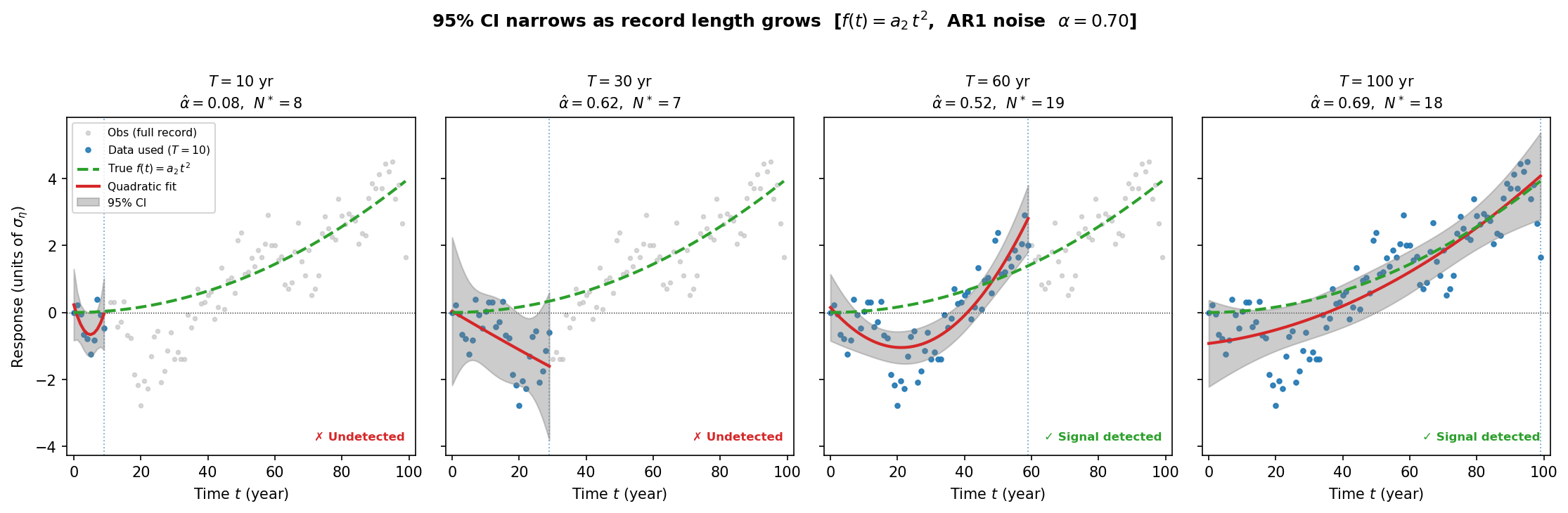
Fig. 1 95% CI (gray shading) for a quadratic forced trend \(f(t)=a_2 t^2\) embedded in AR1 noise (\(\alpha=0.70\)). Each panel uses the same single realization (gray dots), with the blue dots indicating the data window used for fitting. The fitted quadratic trend (red) is compared to the true forced response (green dashed), which is exactly zero at \(t=0\). The CI is wide and overlaps zero for short records (\(T=10, 30\) yr — signal undetected), but narrows progressively until the forced response clearly emerges from noise (\(T=60, 100\) yr — signal detected). The CI width uses the hat-matrix leverage inflated by \(\sqrt{T/N^*}\) to account for AR1 autocorrelation.#
This framework was applied to detecting the forced response of atmospheric rivers under greenhouse warming in , who showed that a second-order polynomial fit combined with an AR1 noise model can identify the time of emergence of a forced signal even from a single model realization — without needing a large ensemble.
Example / deeper dive
Connecting back to the linear case
For \(p = 1\) (linear trend), the framework above reduces exactly to the standard t-test for the regression slope:
The nonlinear case is simply the natural generalization: fit a richer model for \(f(t)\), then use the residual AR1 structure to correct the degrees of freedom. The key insight is that SNR, polynomial fitting, AR1 noise, and effective sample size are all part of one unified regression framework.
Theory of Correlation (Pearson’s Correlation)#
Statistical significance of correlations#
The correlation \(r\) between two time series \(x(t)\) and \(y(t)\) gives a measure of how well the two time series vary linearly together. \(-1 \leq r \leq 1\), with numbers closer to \(\pm1\) implying a stronger linear relationship.
We denote the sample correlation as \(r\) and the theoretical true value as \(\rho\).
If \(\rho = 0\), we can use the t-statistic:
Example: testing the hypothesis that \(\rho = 0\)
We have two time series, each of length 20, correlated at \(r = 0.6\). Does this exceed the 95% confidence interval under \(H_0: \rho = 0\)?
We had no prior knowledge of the sign of the correlation, so we use a two-tailed t-test. For \(\nu = N-2 = 18\), the critical value is \(t_c = 2.1\).
Since \(t = 3.18 > t_c = 2.1\), we can reject the null hypothesis.
Example: confidence limits on the true correlation
What are the 95% confidence limits on the true correlation if you drew 21 samples and obtained \(r = 0.8\)?
With \(t_{0.025} = 2.1\) (for \(\nu = 21-3 = 18\)):
Converting back to correlation via \(\rho = \tanh(\mu_Z)\):
The above statistic only works if the underlying distributions are normal, or if \(N\) is large enough for the CLT to apply (roughly \(N > 20\)).
Figure / in-class demonstration
Figure Example: testing_normality_of_correlations.py
If \(\rho \neq 0\), we must use the Fisher-Z Transformation. When the true correlation is not zero, the distribution of \(r\) is not symmetric, so we cannot directly use the normal/t distribution. The Fisher-Z transformation converts \(r\) into a quantity that is approximately normally distributed:
The Fisher-Z statistic is normally distributed with:
The confidence bounds for \(Z\) are:
To convert back from \(\mu_Z\) to the actual correlation \(\rho\):
Comparing two non-zero sample correlations#
To test whether two correlations \(r_1\) (from sample \(N_1\)) and \(r_2\) (from sample \(N_2\)) are significantly different, apply the Fisher-Z to each:
Then use the z-score for the difference of means:
where \(\delta_{1,2} = \mu_1 - \mu_2\) is the hypothesized difference (typically 0 if \(H_0: \rho_1 = \rho_2\)).
Spearman’s rank correlation#
Spearman’s rank correlation is a nonparametric test for whether paired data monotonically co-vary. No normality assumption is needed.
The original data \(x_i\) and \(y_i\) are converted into ranks \(X_i\) and \(Y_i\), and the correlation is computed on the ranks:
When there are duplicate values, ranks are set to the average position. The standard error is:
Significance can be tested using the Fisher-Z test or the t-test (for \(H_0: \rho = 0\)), as for Pearson’s \(r\).
Figure / in-class demonstration
Figure Example: see slides 08_correlation.pdf
Note: a second nonparametric method is Kendall’s Tau Rank Correlation — not covered here.
Autocorrelation & Estimating the Number of Independent Samples#
Thus far, we have assumed that our time series have no intrinsic memory. Now, we will discuss these assumptions and how to determine the true number of degrees of freedom in an autocorrelated data set.
Stationarity#
Stationarity implies that the statistics of a time series (mean and higher-order moments) are independent of time — unchanging in time. In general, we will assume this is the case. This means one should remove any trend in the data before performing the analysis, using the linear regression method discussed above.
Autocorrelation#
The autocovariance function \(\gamma(\tau)\) is the covariance of a time series with itself at lag \(\tau\):
Figure / in-class demonstration
Figure Example: Draw out example of how autocovariance works.
For a time series with integer positions \(k = 1, 2, \dots, N\):
At \(\tau = 0\): \(\gamma(0) = \overline{x'^2} = \text{variance}\).
The autocorrelation \(\rho(\tau)\) is \(\gamma(\tau)\) normalized by \(\gamma(0)\) — simply the correlation of a time series with itself at another time.
Notes:
\(\gamma\) is symmetric about \(\tau = 0\)
\(-1 \leq \rho(\tau) \leq 1\)
\(\rho(0) = 1\)
if the time series is not periodic, \(\rho(\tau) \rightarrow 0\) as \(\tau \rightarrow \infty\)
Figure / in-class demonstration
Figure Example: see slides 08_correlation.pdf
The first-order autoregressive model (AR1 / red noise)#
Also referred to as a “first order Markov process” or “red noise.”
Red noise: “today is like yesterday plus noise”
where:
\(x\) is a standardized variable (zero mean, unit variance)
\(\Delta t\) is the (constant) time interval between data points
\(a \in [0,1]\) measures the memory of the previous state
\(\epsilon(t) \sim \mathcal{N}(0,1)\) is white noise
Deriving \(a\): Multiply both sides by \(x(t-\Delta t)\) and time-average:
Deriving \(b\): Square both sides and time-average:
Autocorrelation of red noise: Multiplying the recursion two steps forward by \(x(t)\) and averaging shows that \(\rho(2\Delta t) = \rho^2(\Delta t)\), and more generally:
The autocorrelation decays exponentially with an e-folding time:
The e-folding time \(T_e\) is the lag at which \(\rho\) drops to \(1/e \approx 0.368\). For example, if \(\Delta t = 1\) day and \(a = \rho(1) = 0.6\), then \(T_e = 2\) days.
White noise#
White noise is the special case of AR1 with \(a = 0\) (i.e. \(\rho(\tau > 0) = 0\)). It has equal power at all frequencies and zero autocorrelation — no memory of previous time steps. In geophysics, white noise is generally assumed to be normally distributed.
Figure / in-class demonstration
Figure Example: correlation_with_memory_examples.py
Side note: diffusion models in machine learning and their connection to AR processes
Diffusion models (also called Denoising Diffusion Probabilistic Models, DDPMs) have become the dominant generative model architecture in machine learning — used for image synthesis, weather downscaling, and bias correction. They belong in this chapter for a specific reason, not as a digression: the process that destroys the data is an AR(1) process, and the process that rebuilds it is a least-squares regression. Both halves of the algorithm are objects you have already met. The rest is engineering.
How to read this note. Sections 1–3 build the forward process, 4–9 derive the training loss, and 10 states the algorithm. That run is self-contained and strictly linear: if you only want to implement a DDPM, stop at 10. Sections 11–16 then re-read the trained network as a density estimate and apply it to downscaling — which is what you need in order to interpret or modify one.
Companion: the full derivation
Sections 1–10 below follow DDPM: A Complete Derivation step for step, and the numbering matches. The companion note carries every intermediate line that is compressed here: the induction for the closed-form forward marginal, the telescoping ELBO decomposition (Appendix A of Ho et al., 2020), the term-by-term matching of the true posterior, the Gaussian KL identity, and the noise reparameterisation.
Notation — the symbols change meaning here
Machine learning uses \(x\) and \(y\) in the opposite sense to the regression sections above. Statistics fixed \((x,y) = (\text{predictor},\text{response})\); generative ML fixed \(\mathbf{x} = \) the field being modelled and \(\mathbf{y} = \) the conditioning information. Both are entrenched, so this note keeps the ML convention — every diffusion paper you go on to read will use it — but you must hold the mapping in mind:
in the regression sections above |
in this side note |
|
|---|---|---|
the thing you are given (predictor) |
\(x\) |
\(\mathbf{y}\) |
the thing you want (predictand) |
\(y\) |
\(\mathbf{x}_0\) |
what the subscript \(t\) means |
physical time |
index of the noise ladder, \(0\dots T\) |
So \(\mathbb{E}[y\mid x]\) in the regression sections and \(\mathbb{E}[\mathbf{x}_0\mid\mathbf{y}]\) here denote the same operation — the letters are simply exchanged.
Symbols used below
symbol |
meaning |
shape |
|---|---|---|
\(\mathbf{x}_0\) |
the clean high-resolution field you want |
e.g. 1 km precipitation, \(10^4\)–\(10^6\) values |
\(\mathbf{x}_t\) |
that same field after \(t\) noising steps |
always the same shape as \(\mathbf{x}_0\) |
\(\mathbf{y}\) |
the coarse field you actually have |
e.g. 25 km GCM output, far fewer values |
\(t\) |
position on the noise ladder, not time |
\(0\) (clean) to \(T\) (pure noise) |
A six-point example. Let the high-resolution truth be \(\mathbf{x}_0 = [\,2.1,\ -0.4,\ 1.3,\ -1.8,\ 0.6,\ -2.2\,]\), and let the coarse model resolve only blocks of three, so it reports block means \(\mathbf{y} = [\,1.00,\ -1.13\,]\). The noising ladder is then
\(t\) |
\(\sqrt{\bar\alpha_t}\) |
\(\mathbf{x}_t\) |
|---|---|---|
0 |
1.00 |
\([2.10,\ -0.39,\ 1.31,\ -1.81,\ 0.60,\ -2.21]\) |
100 |
0.88 |
\([2.12,\ -0.38,\ 1.50,\ -2.47,\ 1.28,\ -1.98]\) |
250 |
0.45 |
\([1.55,\ -0.30,\ 0.25,\ -0.40,\ 1.01,\ -1.17]\) |
399 |
0.13 |
\([0.13,\ 0.63,\ -0.69,\ -1.74,\ 0.47,\ -0.96]\) |
Three things to notice: \(\mathbf{y}\) never appears in that table — it is never noised, and is supplied unchanged to the network at every reverse step; \(\mathbf{x}_t\) is never a 2-vector, because the subscript changes the noise level, not the resolution; and \(t\) is not time. The task is to produce a plausible 6-vector whose block means are \([1.00,-1.13]\) and whose fine structure looks like real data. Infinitely many exist — which is why we sample rather than solve.
In conditional_diffusion_demo.py these are exactly the variables x0, yobs = A @ x0, and the running x inside ddpm_sample.
Part A — The forward process (how the data is destroyed)
1. The naive forward process, and why it fails
The obvious way to destroy a field is to keep adding noise to it:
Unrolling the recursion gives \(\mathbf{x}_t = \mathbf{x}_0 + \sqrt{\beta}\,(\boldsymbol{\epsilon}_1+\cdots+\boldsymbol{\epsilon}_t)\), and a sum of \(t\) independent \(\mathcal{N}(\mathbf{0},\beta\mathbf{I})\) variables is \(\mathcal{N}(\mathbf{0},t\beta\mathbf{I})\), so
The mean never moves off \(\mathbf{x}_0\) and the variance grows without bound. This is the variance-exploding process, and it is useless for generation: there is no fixed distribution to start sampling from. To draw \(\mathbf{x}_T\) you would already have to know \(\mathbf{x}_0\) — which is the thing you were trying to generate.
2. The variance-preserving forward process
The fix is to shrink the state slightly before adding the noise:
where \(\beta_t\in(0,1)\) is a noise schedule, a small pre-defined sequence that increases with \(t\).
Why \(\sqrt{1-\beta_t}\), and not something else? Take the variance of both sides, exactly as we did for red noise above. If \(\operatorname{Var}(\mathbf{x}_{t-1})=1\) then
The coefficient is precisely what holds the variance fixed — hence variance preserving. This is the AR(1) normalisation of this chapter, term for term. Writing the chapter’s \(x(t) = a\,x(t-\Delta t) + b\,\epsilon(t)\) alongside it, \(a_t = \sqrt{1-\beta_t}\) and \(b_t = \sqrt{\beta_t}\), and the relation \(a^2+b^2=1\) that gave us \(b=\sqrt{1-a^2}\) is the identity being used here. A diffusion model’s forward pass is an AR(1) process with a time-varying memory coefficient, nothing more.
Define
Closed form: jumping straight to step \(t\). By induction (substitute the \(t-1\) result into the recursion), the two independent Gaussian contributions combine with variance \(\alpha_t(1-\bar\alpha_{t-1}) + (1-\alpha_t) = 1-\bar\alpha_t\), giving
This is the telescoping property of AR(1): \(\sqrt{\bar\alpha_t}\) plays exactly the role of \(a^n\), the \(n\)-step autocorrelation, in the notation above. For constant \(\beta\), \(\bar\alpha_t = (1-\beta)^t \to 0\), so the mean tends to \(\mathbf{0}\) and the variance to \(1\):
regardless of what \(\mathbf{x}_0\) was. Two consequences matter: there is now a fixed distribution to start sampling from, and training never has to run the chain — any noise level is one line of arithmetic away.
3. Forward and reverse joint distributions
Because the forward process is a Markov chain, the whole path factorises:
This is fixed and known — it contains no parameters and nothing is learned about it. The reverse process is a second Markov chain, started from pure noise, whose transitions the network must supply:
The difficulty is that the true single reverse step \(q(\mathbf{x}_{t-1}\mid\mathbf{x}_t)\) is intractable: undoing one noising step requires knowing the distribution of all the data that could have produced \(\mathbf{x}_t\). So each reverse transition is modelled as a Gaussian whose mean a neural network provides. Sections 4–9 determine what that network should be trained to output.
Part B — Where the training loss comes from
4. From negative log-likelihood to the ELBO
We want the model to assign high likelihood to real data, i.e. to minimise \(-\log p_\theta(\mathbf{x}_0)\). Marginalising,
which sums over every path from noise to \(\mathbf{x}_0\) and cannot be computed. The standard remedy is to multiply and divide by the known forward process,
and then apply Jensen’s inequality. Since \(-\log\) is convex, \(-\log\mathbb{E}[Y] \le \mathbb{E}[-\log Y]\), so
\(L\) is an upper bound on the negative log-likelihood; equivalently \(-L\) is a lower bound on the log-likelihood, the evidence lower bound (ELBO). Minimising \(L\) is what we can actually do.
5. Rewriting the ELBO as KL divergences
\(L\) as written is still an expectation over whole paths. Four steps turn it into a sum of per-step terms.
Step 1 — expand. Substituting both factorisations,
and separate the \(t=1\) term from the rest.
Step 2 — flip the forward step with Bayes’ rule. By the Markov property \(q(\mathbf{x}_t\mid\mathbf{x}_{t-1}) = q(\mathbf{x}_t\mid\mathbf{x}_{t-1},\mathbf{x}_0)\), and then
This is the key move of the whole derivation. The intractable reverse step \(q(\mathbf{x}_{t-1}\mid\mathbf{x}_t)\) has been replaced by \(q(\mathbf{x}_{t-1}\mid\mathbf{x}_t,\mathbf{x}_0)\), which is tractable — conditioning on the clean starting point makes the exact reverse step available in closed form (section 6).
Step 3 — telescope. The extra ratio introduced by Step 2 collapses:
and the \(q(\mathbf{x}_1\mid\mathbf{x}_0)\) factors cancel against the \(t=1\) term held back in Step 1.
Step 4 — recognise KL divergences. Each surviving log-ratio involves only a few variables, and averaging over the rest turns it into a KL divergence:
Dropping terms. \(L_T\) contains no trainable parameters — it only says the forward chain should end near \(\mathcal{N}(\mathbf{0},\mathbf{I})\), which the schedule already guarantees. \(L_0\) concerns the final, nearly noise-free step and carries little learning signal; it is dropped in practice (the paper models it with a separate discrete decoder). What remains is the sum of \(L_{t-1}\) terms, and every one of them compares two Gaussians.
6. The true posterior \(q(\mathbf{x}_{t-1}\mid\mathbf{x}_t,\mathbf{x}_0)\)
By Bayes’ rule, \(q(\mathbf{x}_{t-1}\mid\mathbf{x}_t,\mathbf{x}_0)\propto q(\mathbf{x}_t\mid\mathbf{x}_{t-1})\,q(\mathbf{x}_{t-1}\mid\mathbf{x}_0)\). Both factors are known Gaussians, so up to an additive constant the log-density is
This is quadratic in \(\mathbf{x}_{t-1}\), so the posterior is itself Gaussian, \(\mathcal{N}(\tilde{\boldsymbol{\mu}}_t,\tilde\beta_t\mathbf{I})\). Matching against \(-\tfrac{1}{2\tilde\beta_t}\|\mathbf{x}_{t-1}-\tilde{\boldsymbol{\mu}}_t\|^2\) term by term:
Variance — from the coefficient of \(\|\mathbf{x}_{t-1}\|^2\),
Mean — from the term linear in \(\mathbf{x}_{t-1}\),
The exact reverse step is a weighted combination of where you are now and where you started — which is why it is only available when \(\mathbf{x}_0\) is known, and why Step 2 of section 5 was necessary.
7. The Gaussian KL reduces to a squared distance
Model the network’s reverse step as \(p_\theta(\mathbf{x}_{t-1}\mid\mathbf{x}_t) = \mathcal{N}\big(\boldsymbol{\mu}_\theta(\mathbf{x}_t,t),\,\sigma_t^2\mathbf{I}\big)\) with \(\sigma_t^2\) fixed, not learned (the paper uses \(\sigma_t^2=\beta_t\) or \(\tilde\beta_t\)). For isotropic Gaussians in \(d\) dimensions,
Both variances are fixed, so the first group is a constant and only the mean term depends on \(\theta\):
A divergence between distributions has become a squared error between two means. This is the same fact that makes least squares the natural loss under Gaussian errors, which is why the chapter’s \(Q=\sum(\hat y_i-y_i)^2\) reappears here unchanged.
8. Reparameterising in terms of noise
The closed form for \(\tilde{\boldsymbol{\mu}}_t\) is an awkward mixture of \(\mathbf{x}_0\) and \(\mathbf{x}_t\), and the network never sees \(\mathbf{x}_0\). But the closed-form forward marginal of section 2 can be rearranged,
Substituting this into \(\tilde{\boldsymbol{\mu}}_t\) and using \(\sqrt{\bar\alpha_{t-1}}/\sqrt{\bar\alpha_t} = 1/\sqrt{\alpha_t}\), the coefficient of \(\mathbf{x}_t\) collapses to \(1/\sqrt{\alpha_t}\) and the coefficient of \(\boldsymbol{\epsilon}\) to \(-\beta_t/(\sqrt{\alpha_t}\sqrt{1-\bar\alpha_t})\):
The network sees \(\mathbf{x}_t\) but not \(\boldsymbol{\epsilon}\), so we give its mean the same functional form and let it supply only the noise term:
Subtracting the two, the \(\mathbf{x}_t\) terms are identical and cancel:
so that
9. Random time steps and the simplified loss
Summing over all \(T\) steps for every training sample is expensive. Since \(\sum_{t=1}^{T}f(t) = T\,\mathbb{E}_{t\sim U\{1,\dots,T\}}[f(t)]\), drawing one random \(t\) per sample gives an unbiased estimate of the full objective. DDPM additionally sets the \(t\)-dependent prefactor to 1, which in practice trains better:
Minimising a divergence between complicated distributions has collapsed into a single sentence: add noise you generated yourself, then ask the network to guess what it was. Because you generated it, the right answer is free, and the intractable path integral of section 4 never appears anywhere in the training code. That — not the noise-adding, which is trivial — is the engineering insight behind diffusion models.
One remark worth making to a class: discarding the prefactor \(\beta_t^2/[2\sigma_t^2\alpha_t(1-\bar\alpha_t)]\) means \(L_{\text{simple}}\) is an unweighted least-squares fit across noise levels, whereas the ELBO prescribes a weighted one. This is the same weighted-versus-unweighted choice met in ordinary regression; here the unweighted version de-emphasises the very small-\(t\) terms and is found to train better.
Part C — The algorithm
10. Training and sampling
Everything above reduces to two short loops. Training — repeat until converged:
Sample \(\mathbf{x}_0\sim p(\mathbf{x})\), \(t\sim U\{1,\dots,T\}\), \(\boldsymbol{\epsilon}\sim\mathcal{N}(\mathbf{0},\mathbf{I})\).
Form \(\mathbf{x}_t = \sqrt{\bar\alpha_t}\,\mathbf{x}_0+\sqrt{1-\bar\alpha_t}\,\boldsymbol{\epsilon}\).
Take a gradient step on \(\nabla_\theta\|\boldsymbol{\epsilon}-\boldsymbol{\epsilon}_\theta(\mathbf{x}_t,t)\|^2\).
Sampling — start from \(\mathbf{x}_T\sim\mathcal{N}(\mathbf{0},\mathbf{I})\), then for \(t=T,\dots,1\):
Draw \(\mathbf{z}\sim\mathcal{N}(\mathbf{0},\mathbf{I})\) if \(t>1\), else set \(\mathbf{z}=\mathbf{0}\).
Update
and return \(\mathbf{x}_0\). Typically \(T=1000\).
Note that the sampler is not a separate construction: that update is exactly \(\boldsymbol{\mu}_\theta\) from section 8 plus a small amount of fresh noise — the learned posterior mean of section 6. The network \(\boldsymbol{\epsilon}_\theta\) is usually a U-Net, but nothing in the derivation depends on that choice; it is simply a flexible regression function.
Part D — What the network has actually learned
Sections 1–10 are the variational route (Ho et al., 2020), and they answer why the training loss takes the form it does. They do not answer what the trained network is. For that there is a second, independently developed route — score matching (Vincent, 2011; Song & Ermon, 2019) — which was only later shown to describe the same algorithm (Song et al., 2021).
The distinction is one this chapter has already drawn once, about the regression slope. You can define \(a_1\) operationally, as the number that minimises \(Q=\sum(\hat y_i - y_i)^2\) — correct, but it tells you nothing beyond the recipe. The result \(a_1 = \overline{x'y'}/\overline{x'^2}\) instead says what \(a_1\) is: a property of the joint distribution, independent of the fitting procedure. In the same way, \(L_{\text{simple}}\) defines \(\boldsymbol{\epsilon}_\theta\) operationally; the sections below say what \(\boldsymbol{\epsilon}_\theta\) is.
11. The noisy data distribution \(p_t\) is a kernel density estimate
To run the reverse process, the network must know which direction makes a noisy field look more like real data. That direction is the score, \(\nabla_{\mathbf{x}}\log p_t(\mathbf{x}_t)\) — the gradient of the log-density of “the distribution of the data after \(t\) steps of noise.” A fair question is who decides what that distribution is. The answer is that nobody does — it is not chosen, it is a consequence. You only ever pick two things:
your data (the training archive: all the precipitation fields you have), and
your noise schedule \(\beta_t\) (how much noise to add at each step).
Once those are fixed, \(p_t\) is completely determined: take every field in your archive, shrink it, add the prescribed Gaussian noise, and look at the spread of everything you get. Formally that is an integral, with \(q\) the closed-form marginal of section 2:
So \(p_t\) is a blurred copy of the real data distribution, and \(t\) controls how blurred. At \(t=0\) there is no blur and \(p_t\) is the data itself; at \(t=T\) every trace is gone and \(p_t\) is plain \(\mathcal{N}(\mathbf{0},\mathbf{I})\). Everything in between is a partially recognisable version of the data — like a photograph going progressively out of focus.
It is a kernel density estimate. With a finite archive of \(n\) fields, the integral is just a sum of Gaussian bumps centred on the (shrunken) training samples:
That is exactly a Gaussian KDE with bandwidth \(h_t = \sqrt{1-\bar\alpha_t}\). The diffusion timestep is a bandwidth knob. Sampling starts from an enormously over-smoothed density — so blurry that the only information left is roughly where the data lives — and sharpens the bandwidth step by step. This is why the reverse process is run gradually rather than in one jump: each step only has to solve an easy, slightly-less-blurry problem.
Crucially, you never have to know \(p_t\). The integral cannot be computed for real data, but section 9 showed that the training rule requires only noise you generated yourself. In conditional_diffusion_demo.py the data distribution is deliberately chosen to be AR1 red noise, i.e. a Gaussian. A Gaussian blurred by a Gaussian is still Gaussian, so there the integral does close, giving \(p_t = \mathcal{N}(\mathbf{0},\ \bar\alpha_t\Sigma + (1-\bar\alpha_t)\mathbf{I})\). That is why the demo needs no training at all — it can write down the exact answer a real network would have to learn.
A caveat that follows from the KDE view
If the network learned the score of \(p_t\) perfectly, it would reproduce the training fields exactly and generate nothing new — because the score of a KDE points back at the samples used to build it. Real diffusion models generalise only because a finite network cannot fit that target exactly. Perfect optimisation of the training objective would be memorisation; useful generation is a controlled failure to reach it. This is worth remembering before trusting a generative downscaling product to produce genuinely unseen extremes.
12. \(\boldsymbol{\epsilon}_\theta\) is an estimate of the score
The bridge from \(L_{\text{simple}}\) to the score is two lines of calculus followed by a result already proved in this chapter.
Step 1 — if you knew \(\mathbf{x}_0\), it is just the derivative of a Gaussian. Recall \(\boldsymbol{\epsilon} = (\mathbf{x}_t - \sqrt{\bar\alpha_t}\mathbf{x}_0)/\sqrt{1-\bar\alpha_t}\). For a known starting point, \(q(\mathbf{x}_t\mid\mathbf{x}_0)\) is an ordinary Gaussian, so
Nothing deep has happened: the gradient of a Gaussian log-density is (mean − point)/variance, and that displacement is the noise that was added, up to scaling.
Step 2 — average over which \(\mathbf{x}_0\) it might have been. Differentiating \(p_t(\mathbf{x})=\int p_0(\mathbf{x}_0)q(\mathbf{x}\mid\mathbf{x}_0)\,d\mathbf{x}_0\) and using \(\nabla q = q\,\nabla\log q\) gives
The marginal score is the posterior average of the conditional scores. Substituting Step 1:
Step 3 — why the trained network equals that. \(L_{\text{simple}} = \mathbb{E}\|\boldsymbol{\epsilon}-\boldsymbol{\epsilon}_\theta(\mathbf{x}_t,t)\|^2\) is an ordinary least-squares regression of \(\boldsymbol{\epsilon}\) on \(\mathbf{x}_t\) — and this chapter has already established what least squares returns: the conditional mean of the target given the predictor. Hence the optimum is \(\boldsymbol{\epsilon}_\theta^\star = \mathbb{E}[\boldsymbol{\epsilon}\mid\mathbf{x}_t]\), which is the identity above. Any \(\approx\) is only because a real network has finite capacity and finite training; the identity itself is exact.
This is the punchline worth stating explicitly: the network is doing plain least-squares regression, and the score identity is what makes that regression secretly a density estimate. You never write down \(p_t\), yet minimising a squared error hands you its gradient. Tweedie’s formula follows in one line by applying \(\mathbb{E}[\,\cdot\mid\mathbf{x}_t]\) to \(\mathbf{x}_0=(\mathbf{x}_t-\sqrt{1-\bar\alpha_t}\boldsymbol{\epsilon})/\sqrt{\bar\alpha_t}\):
Computing both sides of the identity independently for the four-mode mixture used in section 14 — the left by finite-differencing the analytic \(\log p_t\), the right by Monte Carlo over \(8\times10^6\) draws — confirms it:
\(t\) |
\(x_t\) |
\(-\sqrt{1-\bar\alpha_t}\,\nabla\log p_t\) |
\(\mathbb{E}[\epsilon\mid x_t]\) |
difference |
|---|---|---|---|---|
50 |
0.80 |
−0.176874 |
−0.176803 |
\(7.1\times10^{-5}\) |
150 |
−1.00 |
−0.139174 |
−0.139960 |
\(7.9\times10^{-4}\) |
250 |
0.30 |
0.164649 |
0.164322 |
\(3.3\times10^{-4}\) |
350 |
1.50 |
1.341690 |
1.341872 |
\(1.8\times10^{-4}\) |
How to read the identity.
It is a change of units. If \(\mathbf{x}\) carries units \([X]\), then \(\nabla_{\mathbf{x}}\log p_t\) has units \([X]^{-1}\), while \(\sigma_t \equiv \sqrt{1-\bar\alpha_t}\) is a standard deviation with units \([X]\). Their product is dimensionless — as \(\boldsymbol{\epsilon}\sim\mathcal{N}(\mathbf{0},\mathbf{I})\) must be. The score and the noise-prediction are the same vector field measured on two different rulers, and \(\sigma_t\) is the exchange rate.
It is a \(z\)-score. Take a single Gaussian \(p=\mathcal{N}(\mu,\sigma_t^2)\):
which is exactly the \(z\)-score from the beginning of the course. So \(\boldsymbol{\epsilon}_\theta(\mathbf{x}_t,t)\) answers: how many standard deviations am I from where the clean data says I should be? For a mixture it is the posterior-weighted average of the \(z\)-scores relative to each candidate origin.
The sign is geometry. \(\nabla\log p_t\) points uphill in density, toward where the data lives; \(\boldsymbol{\epsilon}\) is the kick that pushed you away from it. Same line, opposite arrows. Denoising means stepping along \(-\boldsymbol{\epsilon}_\theta\).
The two sides scale very differently with \(t\), which is the practical content of the formula:
\(t\) |
\(\sigma_t\) |
RMS of \(\nabla\log p_t\) |
RMS of \(\boldsymbol{\epsilon}_\theta\) |
|---|---|---|---|
399 |
0.991 |
0.98 |
0.98 |
200 |
0.801 |
0.80 |
0.64 |
50 |
0.258 |
1.78 |
0.46 |
5 |
0.037 |
3.00 |
0.11 |
1 |
0.016 |
3.03 |
0.05 |
Two limits are worth checking by hand. At \(t=T\), \(p_T=\mathcal{N}(\mathbf{0},\mathbf{I})\) so \(\nabla\log p_T=-\mathbf{x}_T\) and \(\sigma_T\approx1\), giving \(\boldsymbol{\epsilon}_\theta=\mathbf{x}_T\) — correct, since at pure noise everything you see is the noise. At \(t\to0\), \(\boldsymbol{\epsilon}_\theta\to\mathbf{0}\): here \(\mathbf{x}_t\approx\mathbf{x}_0+\sigma_t\boldsymbol{\epsilon}\) with \(\sigma_t\) tiny, so \(\mathbf{x}_t\) pins down \(\mathbf{x}_0\) but says almost nothing about \(\boldsymbol{\epsilon}\). When a predictor carries no information (\(r^2\to0\)) the least-squares prediction collapses to the unconditional mean, which for \(\boldsymbol{\epsilon}\) is zero — ordinary regression shrinkage. Note the score itself does not diverge here, because this \(p_0\) is a smooth mixture; it would diverge for an empirical \(p_0\) built from delta spikes, which is the memorisation regime of section 11.
This also explains a design choice visible in every implementation: one could equally train the network to output \(\mathbf{x}_0\), or the score directly, since all three are related by the algebra above. Predicting \(\boldsymbol{\epsilon}\) is preferred because its target has unit variance at every \(t\), keeping the regression well-conditioned — the same reason one standardises predictors before a multiple regression.
13. Why the score reading is worth the trouble: conditioning without retraining
Because the normalising constant vanishes under the gradient, Bayes’ rule becomes addition:
So a single unconditional model, trained once on high-resolution fields, can afterwards be conditioned on coarse model output, station observations or satellite retrievals by attaching the appropriate likelihood at sampling time, with no retraining. In the purely variational picture there is no handle on this: each new observation type means feeding \(\mathbf{y}\) to the network as an input and training a new model. The same view also yields deterministic samplers (20–50 steps rather than 1000) and exact likelihoods.
For downscaling the point is worth remembering: it converts “one trained model per data source” into “one prior, many observation operators” — which is precisely the structure of data assimilation.
Part E — What it is for
14. Watching it happen: a wiggly PDF through both processes
The animation below runs a deliberately non-Gaussian (“wiggly”) distribution all the way out to noise and back. The top panel is the distribution; the bottom panel follows 22 individual particles continuously through the forward pass and then back through the reverse pass.
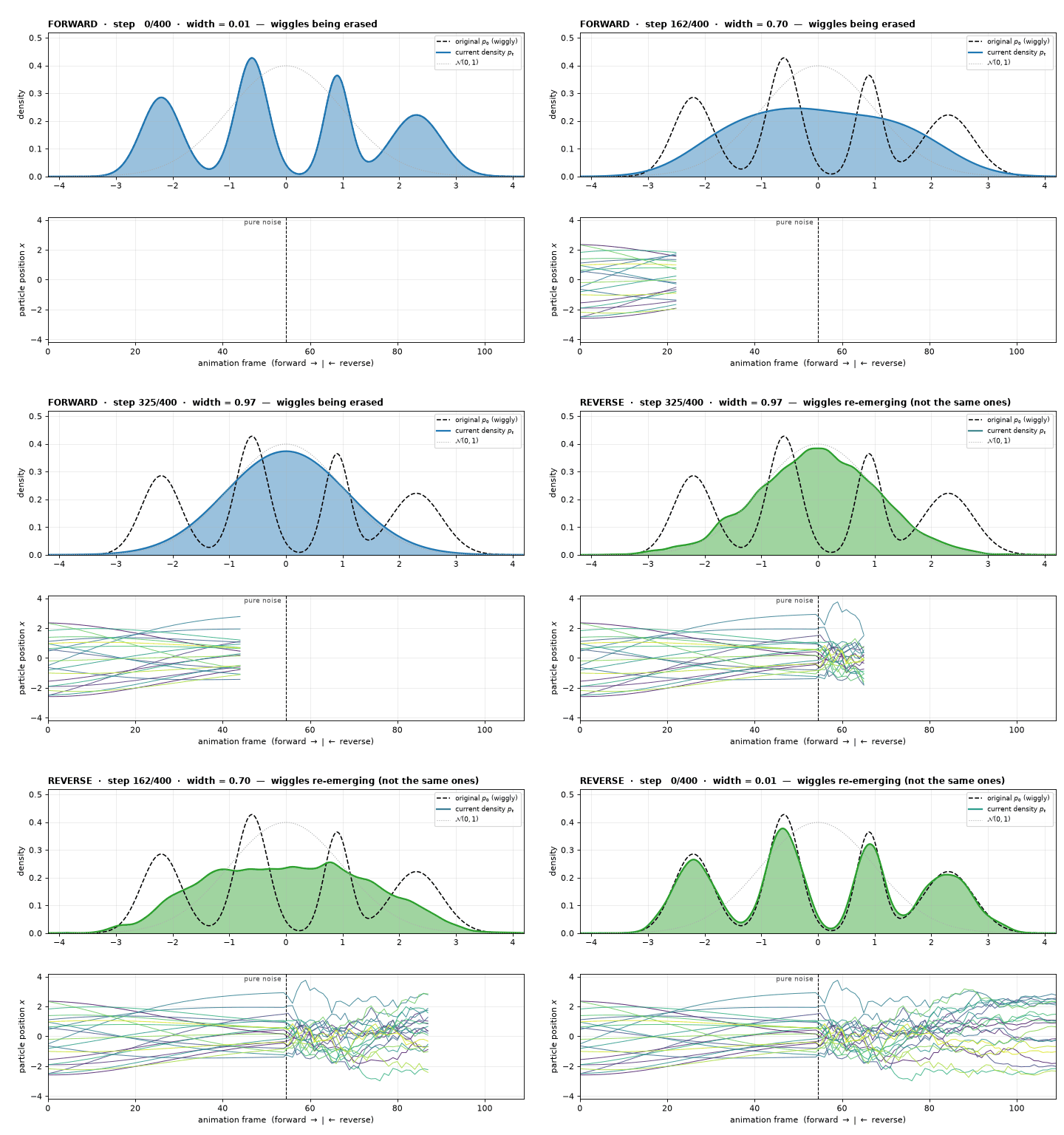
Fig. 2 Forward and reverse diffusion of a four-mode (“wiggly”) PDF. Forward (blue): each bump widens and contracts toward the origin until the four modes have merged into a single indistinguishable \(\mathcal{N}(0,1)\) — the wiggles are erased. Reverse (green): starting from that noise, the wiggles re-emerge and the original shape is recovered. Bottom: the particle paths fan out during the forward pass and re-collapse into the four modes during the reverse pass — but each particle lands in a different mode from the one it started in.#
Three things are worth pointing out to a class:
The forward pass is where the information dies. Watch the two central bumps merge first: they are closest together, so they become indistinguishable earliest. By the time the width reaches \(\approx 1\), no trace of “which bump” survives.
The distribution comes back; the sample does not. Averaged over the tracked particles, the distance between where a particle started and where it ended is \(1.52\) — comparable to the width of the whole distribution. Each particle is reconstructed as a valid draw, not as its own original value. This is the same point taken up in the conditioning discussion below: without \(\mathbf{y}\), there is nothing to say which bump you came from.
The moments are recovered, not memorised. Original: mean \(0.029\), sd \(1.714\), skew \(0.071\), excess kurtosis \(-1.164\). Reconstruction: \(0.040\), \(1.705\), \(0.058\), \(-1.169\).
The static comparison makes the “similar but not identical” point precise, and shows what happens when the score is learned from a finite archive rather than known exactly:
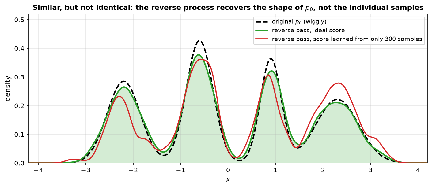
Fig. 3 Black dashed: the true \(p_0\). Green: the reverse pass using the exact score — it recovers the shape faithfully. Red: the reverse pass using a score estimated from only 300 training samples — the fourth mode is too heavy, the first too light, and a spurious bump appears near \(x=-3.3\). The red curve is an honest picture of what a diffusion model trained on a small archive actually gives you.#
A quantitative memorisation check makes the difference concrete. Measuring the mean distance from each generated sample to the nearest training sample, and comparing against the same statistic for a genuinely fresh draw from \(p_0\):
sampler |
mean distance to nearest training sample |
|---|---|
fresh draw from \(p_0\) (the benchmark) |
0.0111 |
reverse pass, exact score |
0.0112 |
reverse pass, score from 300 samples |
0.0027 |
The exact-score sampler is statistically indistinguishable from a fresh draw — it is genuinely generating. The finite-archive sampler sits four times closer to its training data than a fresh draw would: it is partly reproducing what it was trained on. Note that an absolute threshold (“within 0.01 of a training point”) would be meaningless here — with 300 points on a line, every number is close to some training sample. The benchmark comparison is what makes the statistic interpretable.
Full source — diffusion_wiggle_demo.py (click to expand)
"""
diffusion_wiggle_demo.py
========================
Animated illustration of the forward and reverse diffusion processes,
starting from a deliberately "wiggly" (multi-modal, strongly non-Gaussian) PDF.

  FORWARD   p_0 (wiggly)  --- add noise --->  N(0,1)
  REVERSE   N(0,1)        --- denoise    --->  p_0-like, but NOT identical

Two things are animated simultaneously:

  top    the DISTRIBUTION.  Forward is drawn analytically (a Gaussian mixture
         blurred by a Gaussian is still a Gaussian mixture); reverse is the
         kernel density estimate of the particle ensemble.
  bottom individual PARTICLE TRAJECTORIES, carried continuously through the
         forward pass and then back.  A particle does NOT return to where it
         started -- the forward process destroyed that information.

The reverse process uses the empirical (KDE) score of a FINITE training
archive, with a floor on the kernel width to mimic the limited capacity of a
real neural network.  This is why the reconstruction is close to the original
density but visibly smoother -- exactly the memorisation/generalisation
trade-off discussed in the notes.

Outputs: diffusion_wiggle_demo.gif  and  diffusion_wiggle_demo.png
"""
import numpy as np
import matplotlib.pyplot as plt
from matplotlib.animation import FuncAnimation, PillowWriter

rng = np.random.default_rng(4)

# ── The "wiggly" target distribution: a 4-component Gaussian mixture ─────────
W  = np.array([0.25, 0.30, 0.20, 0.25])      # weights
MU = np.array([-2.2, -0.6,  0.9,  2.3])      # means
SD = np.array([0.35, 0.28,  0.22, 0.45])     # std devs

def p0_pdf(x):
    return sum(w * np.exp(-(x-m)**2/(2*s**2)) / (s*np.sqrt(2*np.pi))
               for w, m, s in zip(W, MU, SD))

def p0_sample(k):
    c = rng.choice(len(W), size=k, p=W)
    return MU[c] + SD[c] * rng.standard_normal(k)

# ── Diffusion schedule (same convention as the notes) ────────────────────────
T     = 400
beta  = np.linspace(1e-4, 0.02, T)
alph  = 1.0 - beta
abar  = np.cumprod(alph)

def pt_pdf(x, t):
    """Analytic forward density: mixture blurred by the Gaussian kernel."""
    a = abar[t]
    return sum(w * np.exp(-(x-np.sqrt(a)*m)**2/(2*(a*s**2+1-a)))
               / np.sqrt(2*np.pi*(a*s**2+1-a))
               for w, m, s in zip(W, MU, SD))

# ── The score ────────────────────────────────────────────────────────────────
# (a) IDEAL model: exact score of the true mixture.  A Gaussian mixture blurred
#     by a Gaussian is still a Gaussian mixture, so this is available in closed
#     form -- no training required.  Used for the animation.
def eps_ideal(x, t):
    a  = abar[t]
    v  = a*SD**2 + (1-a)                       # per-component variance at time t
    mu = np.sqrt(a)*MU
    lg = -0.5*(x[:, None]-mu[None, :])**2/v[None, :] \
         - 0.5*np.log(2*np.pi*v)[None, :] + np.log(W)[None, :]
    lg -= lg.max(axis=1, keepdims=True)
    r  = np.exp(lg); r /= r.sum(axis=1, keepdims=True)     # responsibilities
    score = (r*((mu[None, :]-x[:, None])/v[None, :])).sum(1)
    return -np.sqrt(1-a)*score

# (b) TRAINED-ON-FINITE-DATA model: exact score of an archive of N_TRAIN
#     samples.  Used only for the static comparison figure, to show that a
#     finite archive reconstructs a slightly different density.
N_TRAIN = 300
X_TRAIN = p0_sample(N_TRAIN)

def eps_finite(x, t):
    a  = abar[t]
    s2 = max(1.0 - a, 1e-8)
    d2 = (x[:, None] - np.sqrt(a)*X_TRAIN[None, :])**2
    lw = -d2/(2*s2)
    lw -= lw.max(axis=1, keepdims=True)
    w  = np.exp(lw); w /= w.sum(axis=1, keepdims=True)
    x0hat = w @ X_TRAIN                        # E[x0 | xt] = weighted average
    return (x - np.sqrt(a)*x0hat) / np.sqrt(s2)

eps_model = eps_ideal

# ── Run forward, then reverse, storing snapshots ─────────────────────────────
K      = 4000            # particles for the density estimate
N_TRAJ = 22              # particles whose paths we draw
F_FRAMES, R_FRAMES = 55, 55
f_ts = np.linspace(0, T-1, F_FRAMES).astype(int)          # forward snapshots
r_ts = np.linspace(T-1, 0, R_FRAMES).astype(int)          # reverse snapshots

x_start = p0_sample(K)

# forward: closed form, no loop needed
fwd = [np.sqrt(abar[t])*x_start + np.sqrt(1-abar[t])*rng.standard_normal(K)
       for t in f_ts]
# use a single consistent noise draw for the trajectory particles so their
# forward paths look continuous rather than jittery
e_traj = rng.standard_normal(N_TRAJ)
fwd_traj = np.array([np.sqrt(abar[t])*x_start[:N_TRAJ] + np.sqrt(1-abar[t])*e_traj
                     for t in f_ts])

# reverse: start from where the forward pass ended
x = fwd[-1].copy()
x[:N_TRAJ] = fwd_traj[-1]
rev, rev_traj, snap = [], [], set(r_ts.tolist())
store = {}
for t in range(T-1, -1, -1):
    e  = eps_model(x, t)
    mu = (x - beta[t]/np.sqrt(1-abar[t])*e) / np.sqrt(alph[t])
    if t > 0:
        var = beta[t]*(1-abar[t-1])/(1-abar[t])
        x = mu + np.sqrt(var)*rng.standard_normal(K)
    else:
        x = mu
    if t in snap:
        store[t] = x.copy()
rev      = [store[t] for t in r_ts]
rev_traj = np.array([store[t][:N_TRAJ] for t in r_ts])

def kde(samples, grid, bw=0.13):
    d = (grid[:, None] - samples[None, :])/bw
    return np.exp(-0.5*d**2).sum(1)/(len(samples)*bw*np.sqrt(2*np.pi))

# ── Figure / animation ───────────────────────────────────────────────────────
grid = np.linspace(-4.2, 4.2, 400)
p0_curve = p0_pdf(grid)

fig, (axd, axt) = plt.subplots(2, 1, figsize=(9.0, 6.4),
                               gridspec_kw={'height_ratios': [1.15, 1]})

axd.set_xlim(grid[0], grid[-1]); axd.set_ylim(0, 0.52)
axd.set_ylabel('density', fontsize=10); axd.grid(alpha=0.25)
ref,  = axd.plot(grid, p0_curve, 'k--', lw=1.4, label='original $p_0$ (wiggly)')
fillc = [axd.fill_between(grid, p0_curve, color='#1f77b4', alpha=0.55)]
curve,= axd.plot(grid, p0_curve, color='#1f77b4', lw=2.0, label='current density $p_t$')
gauss,= axd.plot(grid, np.exp(-grid**2/2)/np.sqrt(2*np.pi), color='#aaaaaa',
                 lw=1.0, ls=':', label='$\\mathcal{N}(0,1)$')
axd.legend(fontsize=8, loc='upper right', ncol=1)
ttl = axd.set_title('', fontsize=11, fontweight='bold', loc='left')

n_tot = F_FRAMES + R_FRAMES
axt.set_xlim(0, n_tot-1); axt.set_ylim(-4.2, 4.2)
axt.set_xlabel('animation frame  (forward $\\rightarrow$ | $\\leftarrow$ reverse)', fontsize=10)
axt.set_ylabel('particle position $x$', fontsize=10); axt.grid(alpha=0.25)
axt.axvline(F_FRAMES-0.5, color='k', lw=1.0, ls='--')
axt.text(F_FRAMES-1.5, 3.7, 'pure noise', ha='right', fontsize=8, color='#444444')
lines = [axt.plot([], [], lw=0.9, alpha=0.85,
                  color=plt.cm.viridis(i/N_TRAJ))[0] for i in range(N_TRAJ)]
traj_all = np.vstack([fwd_traj, rev_traj])       # (n_tot, N_TRAJ)

HOLD = 8
def update(k):
    # map animation index -> (phase, snapshot index) with holds at each end
    if k < F_FRAMES:
        ph, i = 'fwd', k
    elif k < F_FRAMES + HOLD:
        ph, i = 'fwd', F_FRAMES-1
    elif k < F_FRAMES + HOLD + R_FRAMES:
        ph, i = 'rev', k - F_FRAMES - HOLD
    else:
        ph, i = 'rev', R_FRAMES-1

    if ph == 'fwd':
        t = f_ts[i]; y = pt_pdf(grid, t); col = '#1f77b4'
        ttl.set_text(f'FORWARD  ·  step {t:3d}/{T}  ·  width = {np.sqrt(1-abar[t]):.2f}'
                     '  —  wiggles being erased')
        j = i
    else:
        t = r_ts[i]; y = kde(rev[i], grid); col = '#2ca02c'
        ttl.set_text(f'REVERSE  ·  step {t:3d}/{T}  ·  width = {np.sqrt(1-abar[t]):.2f}'
                     '  —  wiggles re-emerging (not the same ones)')
        j = F_FRAMES + i

    curve.set_data(grid, y); curve.set_color(col)
    fillc[0].remove()
    fillc[0] = axd.fill_between(grid, y, color=col, alpha=0.45)
    for m, ln in enumerate(lines):
        ln.set_data(np.arange(j+1), traj_all[:j+1, m])
    return [curve, fillc[0], ttl, *lines]

n_frames = F_FRAMES + HOLD + R_FRAMES + HOLD
ani = FuncAnimation(fig, update, frames=n_frames, blit=False, interval=70)
# NB: do not use tight_layout here -- it would be computed while the dynamic
# title is still empty and would leave no room for it.
fig.subplots_adjust(left=0.09, right=0.985, top=0.915, bottom=0.095, hspace=0.30)
ani.save('diffusion_wiggle_demo.gif', writer=PillowWriter(fps=14), dpi=80)
print('Saved: diffusion_wiggle_demo.gif')

# ── Second reverse run, this time with the finite-archive score ─────────────
xf = fwd[-1].copy()
for t in range(T-1, -1, -1):
    e  = eps_finite(xf, t)
    mu = (xf - beta[t]/np.sqrt(1-abar[t])*e) / np.sqrt(alph[t])
    xf = mu + (np.sqrt(beta[t]*(1-abar[t-1])/(1-abar[t]))*rng.standard_normal(K)
               if t > 0 else 0)

# ── Static summary figure: original vs reconstructions ──────────────────────
fig2, ax = plt.subplots(figsize=(9.5, 4.2))
ax.plot(grid, p0_curve, 'k--', lw=2.2, label='original $p_0$ (wiggly)')
ax.plot(grid, kde(rev[-1], grid), color='#2ca02c', lw=2.2,
        label='reverse pass, ideal score')
ax.fill_between(grid, kde(rev[-1], grid), color='#2ca02c', alpha=0.20)
ax.plot(grid, kde(xf, grid), color='#d62728', lw=1.8, ls='-',
        label=f'reverse pass, score learned from only {N_TRAIN} samples')
ax.set_xlim(grid[0], grid[-1]); ax.set_ylim(0, 0.52)
ax.set_xlabel('$x$', fontsize=11); ax.set_ylabel('density', fontsize=11)
ax.set_title('Similar, but not identical: the reverse process recovers the '
             'shape of $p_0$, not the individual samples',
             fontsize=11, fontweight='bold')
ax.legend(fontsize=9); ax.grid(alpha=0.3)
plt.tight_layout()
plt.savefig('diffusion_wiggle_demo.png', dpi=150, bbox_inches='tight')
print('Saved: diffusion_wiggle_demo.png')

# ── Diagnostics ──────────────────────────────────────────────────────────────
start = x_start
print(f"\n{'':32s}{'mean':>8}{'std':>8}{'skew':>8}{'kurt':>8}")
for nm, s in [('original p_0', start), ('reconstructed (ideal)', rev[-1]),
              (f'reconstructed ({N_TRAIN} samples)', xf)]:
    z = (s-s.mean())/s.std()
    print(f"{nm:32s}{s.mean():8.3f}{s.std():8.3f}{(z**3).mean():8.3f}{(z**4).mean()-3:8.3f}")

moved = np.abs(traj_all[0] - traj_all[-1])
print(f"\nTracked particles: mean |start - end| = {moved.mean():.2f}  "
      "(they do NOT return to their starting points)")

# Memorisation check: distance to the nearest TRAINING sample, compared with
# the same statistic for a genuinely fresh draw from p_0.  (An absolute
# threshold is meaningless here -- with N_TRAIN points on the line, every
# number is close to *some* training sample.)
fresh = p0_sample(K)
d_ideal  = np.abs(rev[-1][:, None] - X_TRAIN[None, :]).min(1).mean()
d_finite = np.abs(xf[:, None]      - X_TRAIN[None, :]).min(1).mean()
d_fresh  = np.abs(fresh[:, None]   - X_TRAIN[None, :]).min(1).mean()
print(f"\nMean distance to nearest training sample:")
print(f"   fresh draw from p_0 (the benchmark) : {d_fresh:.4f}")
print(f"   reverse pass, ideal score           : {d_ideal:.4f}")
print(f"   reverse pass, {N_TRAIN}-sample score      : {d_finite:.4f}"
      "   <- ~0 means it is reproducing its training data")
15. Application to downscaling, and why conditioning is necessary
For climate downscaling, \(\mathbf{x}_0\) is a high-resolution field (e.g. 1 km precipitation) and the U-Net is conditioned on a low-resolution field \(\mathbf{y}\) (e.g. 25 km GCM output), so the model learns \(p(\mathbf{x}_0\mid\mathbf{y})\) rather than \(p(\mathbf{x}_0)\).
A natural objection: if the forward process destroys everything, how can the reverse process know what is signal and what is noise? The answer has two parts, and it is worth keeping them separate.
1. The learned prior tells the model what data looks like. By section 12 the trained network is an estimate of the score of \(p_t\), and Tweedie’s formula turns it into \(\mathbb{E}[\mathbf{x}_0\mid\mathbf{x}_t]\). “Signal” is defined as the direction of the training-data manifold. This is why unconditional diffusion models work at all — no conditioning input is required to generate a realistic field. (The network is always conditioned on \(t\), but that only tells it the current noise level.)
2. The conditioning tells the model which realisation. An unconditional model produces a plausible field, never the field behind a particular observation — that information was destroyed in the forward pass, as the particle trajectories in section 14 show directly.
The connection to everything above is exact. Ordinary least squares returns the conditional mean of the predictand given the predictor — written \(\mathbb{E}[y\mid x]\) in the regression sections, and \(\mathbb{E}[\mathbf{x}_0\mid\mathbf{y}]\) in the notation of this note. It is a single best estimate, and its variance is only \(r^2\) times the variance of the target. The residual \((1-r^2)\) fraction is discarded, which is precisely why regression-based downscaling produces fields that are too smooth. A conditional diffusion model learns the full conditional distribution, so it restores that \((1-r^2)\) fraction — not as white noise, but with the spatial and temporal structure learned from data:
what it returns |
variance |
tied to this \(\mathbf{y}\)? |
|
|---|---|---|---|
Unconditional diffusion |
a draw from \(p(\mathbf{x}_0)\) |
correct |
no |
Regression / OLS |
\(\mathbb{E}[\mathbf{x}_0\mid\mathbf{y}]\) |
\(r^2\sigma^2\) — too smooth |
yes |
Conditional diffusion |
a draw from \(p(\mathbf{x}_0\mid\mathbf{y})\) |
correct |
yes |
In short: regression gives the best guess; conditional diffusion gives a plausible draw. The prior narrows the possibilities from “any array of numbers” to “realistic weather”; the conditioning narrows them further to “realistic weather consistent with this particular day.”
Figure / in-class demonstration
Figure: conditional_diffusion_demo.py — a 1-D toy downscaling problem in which the prior is AR1 red noise (\(\alpha=0.85\), \(n=240\)), so the “neural network” \(\boldsymbol{\epsilon}_\theta\) is available in closed form and a genuine DDPM reverse loop can be run with no training. The coarse “GCM” field is the block mean over 12 points, which explains \(r^2 = 0.63\) of the variance.
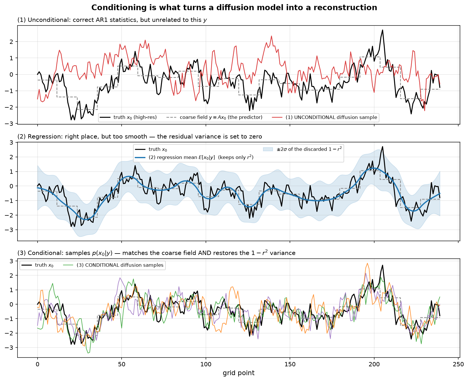
Fig. 4 Unconditional vs. regression vs. conditional reconstruction of an AR1 field from its block means. (1) The unconditional diffusion sample has the correct variance (0.92) but correlates with the truth at only \(+0.002\) — statistically perfect, informationally useless. (2) The regression mean \(\mathbb{E}[x_0|y]\) locates the signal well (corr \(+0.86\)) but its variance is \(0.61 \approx r^2 = 0.63\); the shading shows the discarded \(1-r^2\). (3) Conditional diffusion samples honour the coarse field exactly and recover the full variance (0.96), matching the analytic \(p(x_0|y)\).#
Note that the correlation with the truth drops from 0.86 to 0.66 when the residual variance is added back. The conditional sample is a worse point estimate than the regression mean but a better field, because it has the correct spectrum. This is the same bias–variance trade that motivates using \(\hat y\) for prediction but \(\hat y + \text{residual}\) for anything requiring realistic variability (extremes, thresholds, spatial gradients).
16. Summary: the AR(1) ↔ diffusion dictionary
AR(1) concept |
Diffusion model equivalent |
|---|---|
\(a\) (memory coefficient) |
\(\sqrt{1-\beta_t} = \sqrt{\alpha_t}\), set by the noise schedule |
\(b = \sqrt{1-a^2}\) (noise amplitude) |
\(\sqrt{\beta_t}\) |
\(a^n\) (\(n\)-step autocorrelation) |
\(\sqrt{\bar{\alpha}_t}\) |
unit-variance normalisation \(a^2+b^2=1\) |
the variance-preserving condition of section 2 |
white noise limit (\(a \to 0\)) |
\(\mathbf{x}_T \to \mathcal{N}(\mathbf{0},\mathbf{I})\) as \(T\to\infty\) |
least squares returns \(\mathbb{E}[y\mid x]\) |
\(\boldsymbol{\epsilon}_\theta^\star = \mathbb{E}[\boldsymbol{\epsilon}\mid\mathbf{x}_t]\), hence the score |
fitted part \(y_{\text{fitted}}\) (the \(r^2\) fraction) |
conditional mean \(\mathbb{E}[\mathbf{x}_0\mid\mathbf{y}]\) |
residual \(y_{\text{residual}}\) (the \(1-r^2\) fraction) |
stochastic part of the reverse process |
The key innovation of diffusion models is not the forward AR(1) process — that is just Gaussian noise addition, and you derived its normalisation earlier in this chapter — but the learned reverse process, which turns pure noise back into structured data. The statistical machinery of AR1 and least squares you learned here is the exact mathematical foundation.
Effective sample size \(N^*\)#
Persistence in a data set leads to overestimation of the sample size, because each data point is not independent of its neighbors. If persistence is ignored, the standard error of the mean is underestimated and the t-statistic is inflated.
The solution is to introduce an effective sample size \(N^* \leq N\) and substitute it for \(N\) in formulas.
For a first-order AR process, \(N^*\) can be estimated with the Bretherton/Wilks approximation (Wilks, p. 127):
if \(\rho(1) = 0\) (white noise): \(N^* = N\)
as \(\rho(1)\) increases, \(N^*\) decreases
An equivalent form from Leith (J. Appl. Meteor., 1973):
The factor of 2 reflects the fact that any point in red noise can be predicted by points both before and after it. The Leith formula can also be written as:
The table below shows \(N^*/N\) as a function of lag-1 autocorrelation:
\(\rho(\Delta t)\) |
\(<0.1\) |
\(0.3\) |
\(0.5\) |
\(0.7\) |
\(0.9\) |
|---|---|---|---|---|---|
\(N^*/N\) |
\(\approx 1\) |
\(0.60\) |
\(0.35\) |
\(0.18\) |
\(0.053\) |
Bretherton et al. (J. Climate, 1999) proposed a less conservative approximation (use for variance/higher-order moments):
This yields nearly twice as many degrees of freedom as the Leith formula. For testing the mean, use the Leith formula; for testing variance, the Bretherton formula may be used.
Figure / in-class demonstration
Figure Example: effective_sample_size.py — plot of \(N^*/N\) vs \(\rho(\Delta t)\) comparing the Leith and Bretherton approximations.
Multiple Regression (Multi-linear Regression)#
Basic idea: Generalize the regression coefficient derivation to multiple linear predictors:
The fit now lives in a multi-dimensional predictor space.
Figure / in-class demonstration
Figure Example: 3-D scatter diagram — points \(\hat{y}\) plotted against two orthogonal predictor axes \(X_1\) and \(X_2\), with a best-fit plane drawn through the point cloud.
If \(X_1\) and \(X_2\) are orthogonal (at right angles):
they give independent information
their inner product is 0
if they span the space, they “form a basis”
If \(X_1\) and \(X_2\) are not orthogonal:
they are not independent and share redundant information
The usefulness of independent predictors motivates EOF analysis (to be discussed later).
Generalized normal equations#
For multiple predictors \(x_1, x_2, \dots, x_n\), minimize:
Setting \(\partial Q/\partial a_i = 0\) for \(i = 0, \dots, n\) gives \(n+1\) equations. If the mean has been removed from all variables (\(a_0 = 0\)), the \(j\)th equation is:
In matrix form:
Or compactly: \(C_{x_i x_j}\, a_j = C_{x_i y}\)
Key observations:
The left-hand side \(\mathbf{C}_{xx}\) is the covariance matrix of the predictors (diagonal = variances, off-diagonal = covariances)
The right-hand side \(\mathbf{C}_{xy}\) is the covariance vector between predictors and predictand
If each variable is standardized, \(\mathbf{C}_{xx}\) becomes the correlation matrix and \(\mathbf{C}_{xy}\) the correlation vector
If predictors are linearly independent, off-diagonal elements are 0 and the \(a_j\)’s can be found algebraically
Otherwise, solve via matrix inversion:
Multiple regression — how many predictors should I use?#
Assuming all variables are standardized, the normal equations become \(r(x_i, x_j)\,a_i = r(x_j, y)\). For two predictors:
Solving:
The total fraction of explained variance (\(R^2\)) with two predictors:
Example: does adding a second predictor help?
Say \(r_{1,y} = r_{2,y} = r_{1,2} = 0.5\).
With only \(x_1\): \(R_1^2 = r_{1,y}^2 = 0.25\)
Adding \(x_2\):
Adding \(x_2\) increases the explained variance from 25% to 33%. ✓
Now suppose \(r_{2,y} = 0.25\) (everything else the same):
Adding \(x_2\) adds nothing. The minimum useful correlation for \(x_2\) is:
So \(r_{2,y}\) must exceed 0.25 to be worth adding.
Key guidelines:
Ideal case: \(r_{1,2} = 0\) — two completely independent predictors
Worst case: \(r_{1,2} = 1\) — \(x_2\) provides no new information
Adding too many predictors can lead to overfitting — fitting the noise rather than the signal. Always use as few predictors as possible and test the fit on independent data.
Figure / in-class demonstration
Figure Example: Adjusted \(R^2\) — see https://en.wikipedia.org/wiki/Coefficient_of_determination#Adjusted_R2