Week 1: Predictability of Weather and Climate
Contents
Week 1: Predictability of Weather and Climate
In this week, we will walk through a few fundamental concepts of predictability, including how does it connect to statistics, differential equations and linear algebra. You will find out the definition of predictability is relatively straightforward.
Climatological distribution and forecast distribution
When we say something (let’s say \(x(t)\)) is predictable, that means we can somewhat track its time evolution. However, in most cases, our confidence about what \(x(t)\) should be will decrease with the increase of forecast lead time (defined as the time difference between initial state and the final state). Thus, it is physically more reasonable to use a probability density function (PDF \(p(x(t))\)) to describe \(x(t)\) since we are talking about how “confident” we are.
Now, let’s consider two very extreme cases. The first case is \(t\rightarrow 0\). In this case, we are very certain what \(x(t)\) should be because it is literally the current states or so-called observation. Thus, it’s not hard to find \(p(x(0))\) is narrow and is almost like a delta function (FIG1, solid line). The second case is when \(t\rightarrow \infty\). In this case, we don’t have any confidence. Thus, the best way to estimate \(x(t)\) is by randomly sampling from its historical values (Fig. 1, dashed line, a.k.a. guessing). Thus, from \(t=0\) to \(t\rightarrow \infty\), we can see \(p(x(t))\) is evolving from one PDF to the other. Here we give these two distribution different names. For the one which we use to describe how confident we are is called forecast distribution and the one when forecast lead time approaches infinity is called climatological distribution (also called “population” in statistics).
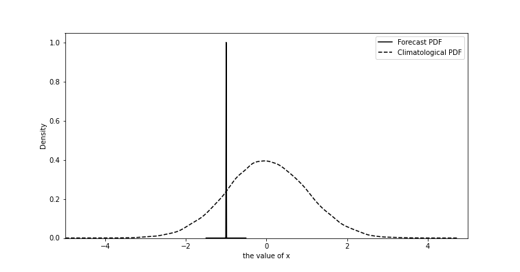
Fig. 1 An example of forecast probability density function and climatological probability density function.
Here we can formulate our mathematical definition of “time of predictability limit”. It is defined as the “moment” that the following null hypothesis is rejected.
(1) tells us that the moment we can no longer tell the difference between \(p(x(t))\) and \(p(x(\infty))\) is also the moment we hit the predictability limit because the best estimation of \(p(x(t))\) is not better than random guess! Now, we can see how predictability connects to statistical test.
Another interesting thing you might have noticed…when we talk about predictability, we don’t use the ground truth, i.e., the observed \(x(t)\). Yes, because the measurement of predictability doesn’t rely on ground truth or observation. Instead, it only relis on the forecast states. This is so-called perfect model assumption and we will have more detailed discussion in week 3.
State-dependent predictability and mathematical assumptions
One interesting fact about predictability is that there is no universal value. You might think…OK that sounds weird and counter-intuitive. For example, we know for typical numerical weather forecast, we will say the predictability limit is around 10 days to 2 weeks. After that, we can no longer trust the model output. However, we will soon realize “10 days to 2 weeks” is only rule of thumb. In some cases, we can even struggle with the low prediction confidence at a forecast lead time of 3 days! Sounds crazy right? Here, let me use the famous Lorenz 63 model to demonstrate what I means.
Note
Lorenz 63 model [Lor63] can be considered as the minimalist model for studying chaos and predictability and it only contains 3 prognostic variables. Indeed, to generate chaotic behavior, the minimum size of independent variables is 3. Smaller than 3, we won’t have chaotic behavior in a dynamical system. We will cover more details about Lorenz model in week 3.
(2) is the Lorenz 63 model with the selected parameters of \(\rho=28\), \(\sigma=10\) and \(\beta=\frac{8}{3}\). This parameter selection makes sure Lorenz 63 model has a chaotic behavior. (The homework assignment will let you test different parameters and see how the dynamical behavior changes.) In this model, we select three different initial states and generate the ensemble simulations by slightly perturbing the initial x,y and z. The result is shown in Fig. 2. We can find in FIG2(a) case, the model spread grows relatively fast and soon diverge into two groups (\(\sim 50\%\) on the right/left). In the second scenario (i.e., FIG2(b)), the difference among ensemble members is small at the very beginning but start to bifurcate later. In the last case (FIG2(c)), different members stay close even at the end of simulation suggesting a relatively small error growth rate.
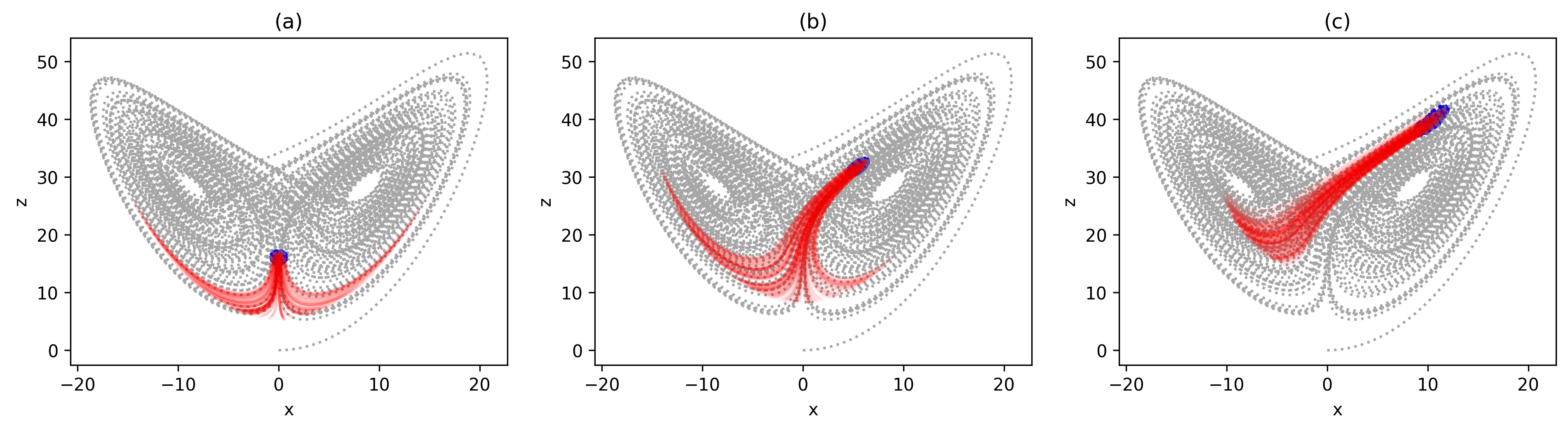
Fig. 2 The three scenarios of ensemble forecasts based on L63 model (a) fast error growth (b) average error growth (c) slow error growth
We can go one step further and plot the forecast PDF (x component) at the final state from three scenarios and the result is shown in FIG3. We also include the climatological PDF as a reference, which is generated by a long-term simulation with 50000 time steps (non-dimensional time). If you still remember what we discuss at the very beginning, the predictability limit is defined by “when” we can reject the null-hypothesis in (1). Thus, by comparing how similar the two distributions are can inform us how predictable the given dynamical system is. In FIG3, we can easily find the forecast PDF in (a) and the climatological PDF are quite similar. However, for cases in (b) and (c), we can still distinguish the forecast PDFs from the climatological PDF indicating we haven’t reached the predictability limit yet.
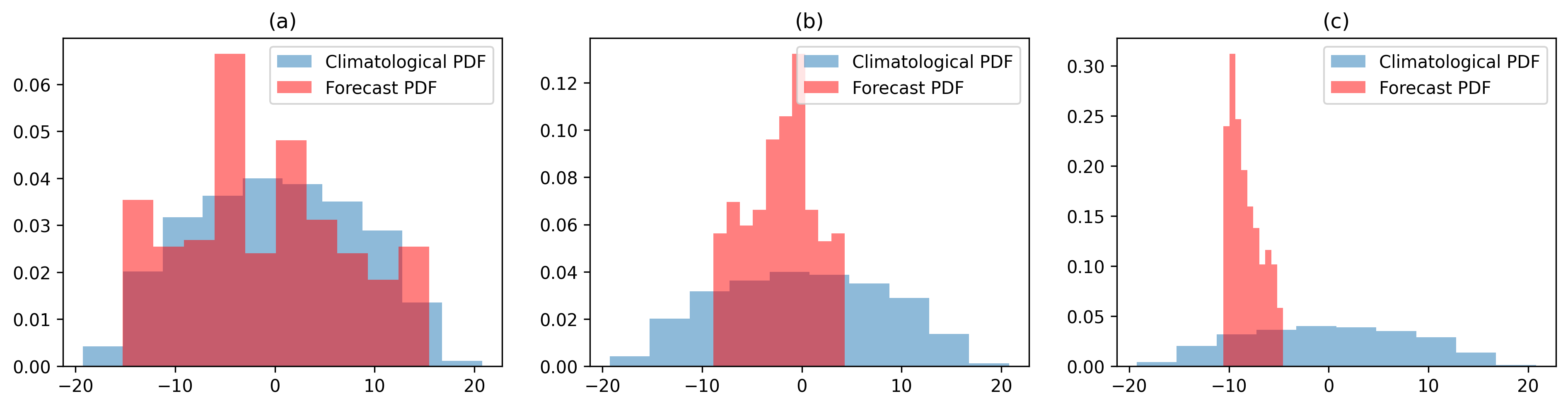
Fig. 3 The final states’ probability density function of three ensemble forecast shown in Fig. 2
One take-home message in FIG2 and FIG3 is, the predictability is a function of state rather than an universal number. Now, we can imagine why the most experienced forecasters and the state-of-art NWP systems can still struggle sometimes…(Thus, be kind to them). There are also a few things to keep in mind. First, we only consider the uncertainty in model initial states but have ignored the uncertainty in model structures (e.g., if the model is correct) or the rounding error. This perfect model assumption is one of the most important assumption in the enrire course (and probably the entire field) since it tells us the upper limit of predictability. It also tells us, as long as we have infinitesimal error in model initial states, the predictability limit is inevitable. Second, predictability has no meaning unless the ensemble simulations are used since its definition is based on how fast one ensemble member can diverge from the other. Third, to reject the null hypothesis in (1), we need to choose a significance level. This indicates that we can always use a very low significance level (e.g., \(1\%\) or \(0.1\%\)) to say we haven’t reached the predictability limit. Thus, clearly define what threshold we are using for testing the null hypothesis is very important.
Where the uncertainties come from?
At the end of previous section, we talk about the potential uncertainties can come from three different places (or at least we can attribute any kind of forecast uncertainty to these three). Of course they can happen at the same time and be indistinguishable in some cases but we will first scrutinize them individually for the purpose of discussion. The first uncertainty is the initial state error or the observational error. In a perfect observation, the spatial and temporal resolution should go all the way down to the smallest scale (molecular scales). Because as long as we have missing observation, the upscale growth of initial error from those regions will ultimately lead to an unpredictable future (if the underlying dynamics is chaotic).
The second error source is from the imperfect model physics. Specifically, the physical parameterizations used to approximate the bulk effect of subgrid-scale processes (i.e., the scales smaller than the model grid) are the major uncertainty source. The details of parameterizations will be discussed in other class and we will briefly walk through the main concept. One main reason of using physical parameterizations is due to the limited computational power. For example, to accurately predict the time evolution of an extratorpical storm, we also need to predict the convection embedded in the frontal structures since the latent heat release by these convections is not negligible. However, explicitly resolving this small-scale thunderstorms is not computationally feasible for the purpose of synoptic weather forecast. Thus, in most NWP systems, we use so-called cumulus parameterizations to approximate the bulk effect of convective cloud. The reason that cumulus parameterization works is that the large-scale environment usually reaches an quasi-equilibrium state with the small scale convection (i.e., coherence exists). Therefore, we can approximate the net convective activity by using the large-scale information. However, similar to the first uncertainty (observational uncertainty), the observational error exists in all spatial scales and thus a PDF (stochastic parameterization) is required to describe the subgrid-scale statistics. While stochastic parameterization seems necessary, it’s not the case in most prevailing NWP systems. In addition to the cumulus parameterization, similar problems also exist in other physical parameterizations.
The last uncertainty is the rounding error. Comparing with the former two uncertainties, rounding error has the least impacts to the weather and climate predictions. Sometimes we can even have some trade-off… i.e., allowing for certain rounding error to save computational time. The main reason we can do that is because the uncertainties from observation and model physics are way bigger (\(>\mathcal{O}(5)\)) than the uncertainty caused by rounding error. More details can be found in [HMPDuben20] and the leading author, Sam Hatfield’s website link.
Note
Lorenz 96 [Lor96] is one of the simplest models attemping to deal with the underpinning theory of subgrid-scale processes, and we will talk about more details in Week 4.
\
Introduction to ensemble forecast in weather and climate
Given the discussion about, we know two facts: (1) ensemble forecast is necessary when talking about predictability and (2) predictability limit is state-dependent. We also use Lorenz 63 model to justify these statements. Now, let’s try to describe both facts in a single formula. First, we can write down the prognostic equations in a more generalized form.
where \(\mathbf{X}\) is the state vector (i.e., [x,y,z]) and F is a nonlinear operator. Here we assume the initial uncertainty is small and F is differentiable. Then (3) leads to (4) and (5).
and
(4) is a linear-tagent function of (3) and \(\mathbf{M}(t,t_0)\) in (5) is a progagator operator (and \(\frac{dF}{d\mathbf{X}}\) is a Jacobian matrix) which maps the initial state of \(\delta\mathbf{X}(t_0)\) to the final state \(\delta\mathbf{X}(t)\). It is important that \(\mathbf{M}(t,t_0)\) is both function of \(t\) and \(t_0\). That means the time evolution of \(\delta\mathbf{X}(t)\) is not only determined by where \(\mathbf{X}\) starts but also depends on where it has been through! You might have noticed this is our fact (2).
By observing (5), we can find the initial error (i.e., the difference between each member) will grow rapidly if \(\int_{t_0}^{t} \frac{dF}{d\mathbf{X}} dt'>0\). An alternative way to describe this phenomena is the prognostic equation of forecast PDF
where \(\rho(\mathbf{X},t)\) is the forecast PDF at given \(\mathbf{X}\) and \(t\) and \(\mathrm{det}{(\mathbf{M}(t,t_0))}\) is the determinant of \(\mathbf{M}(t,t_0)\). Mathematically, a determinant indicates how the area spanned by vectors \(\delta\mathbf{X}\) is scaled after linear transformation. (we will have more discussion in weeks 3-6, also check out the awesome video by 3Blue1Brown !!)
A simple example is
In this case, the \(\mathrm{det}{(\begin{bmatrix} 1 & 0 \\ 0 & 2 \end{bmatrix})}\) equals 2 indicating the area spanned by \(\begin{bmatrix} 1 & 0 \\ 0 & 1 \end{bmatrix}\) will be scaled by 2 after linear transformation. Following a similar vein, from (5), we know the area spanned by \(\delta\mathbf{X}\) will increase by a factor of \(\mathbf{M}(t,t_0)\) indicating the ensemble density (i.e., \(\rho(\mathbf{X},t)\)) will decrease by the same factor due to the conservation law (i.e., total number of ensemble members won’t change). This will lead to equation (6). (6) is a powerful equation since it predicts the forecast PDF and you will see it multiple times in the future. Now, there is only one question left. If we would like to generate reliable ensemble forecast, what kind of initial states \(\mathbf{X}\) should be used for forecast? Practically, we want an ensemble forecast which can cover as many scenarios as possible. Thus, the initial states which can generate the most reliable forecast are usually the states with the largest error growth rate. On the other hand, high error growth rate can also lead the low forecast confidence. Therefore, reaching a balance between the two is important topic in Data Assimilation.
References
- HMPDuben20
Sam Hatfield, Andrew McRae, Tim Palmer, and Peter Düben. Single-precision in the tangent-linear and adjoint models of incremental 4d-var. Monthly Weather Review, 148(4):1541–1552, 2020.
- Lor63
Edward N Lorenz. Deterministic nonperiodic flow. Journal of atmospheric sciences, 20(2):130–141, 1963.
- Lor96
Edward N Lorenz. Predictability: a problem partly solved. In Proc. Seminar on predictability, volume 1. 1996.