Week 2: Predictability source in atmosphere
Contents
Week 2: Predictability source in atmosphere
In this week, we will talk about the potential predictability source in the atmosphere. Before we dig right in, let’s quickly recap what we learned last week. We know the predictability is defined as “when” we can no longer differentiate the forecast distributions and the climatological distribution (i.e., (1)). We also know the error growth, which can be formulated as \(\mathrm{exp} \int_{t_0}^{t} \frac{dF}{d\mathbf{X}} dt'\) (5), strongly depends on where the integration starts and where it has been through (just like our life!). Thus, the most predictable components are usually those components with the longest memory (i.e., \(\int_{t_0}^{t} \frac{dF}{d\mathbf{X}} dt'\) is small).
The origins of predictability (Scale Separation) and balanced dynamics
In a dynamical system, we can use scale analysis to identify the phenomenon with the longest memory and our Earth atmosphere is no exception. The atmosphere can be described by the equations of motion of a fluid.
where \(\mathbf{u}\) is momentum in vector form, \(p\) is pressure, \(\rho\) is density, \(\nu\) is the kinematic viscosity and \(\mathbf{F}\) is the external forces such as gravity. The second equation is the mass conservation, which will show up again in the later section when we talk about the ensemble forecast. The third equation is the thermodynamics equation, where \(\theta\) is the potential temperature, \(c_p\) is the heat capacity of air at a constant pressure, and \(\dot{Q}\) is the diabatic process. The first equation of (8) is so-called Navier-Stokes equation. If we drop the viscosity term, it is called Euler equation. With a few steps of assumptions (i.e., no acoustic wave, hydrostatic and geostrophic balances and beta plane, see Vallis Ch 5.4 for detailed derivations), we can further simplify the model to a single-variable prognostic equation, which describes the time evolution of Rossby wave (9).
The first equation of (9) is quasi-geostrophic vorticity equation, where \(\zeta=\nabla\times\mathbf{u}\), \(v_g\) is the meridional component of the geostrophic wind, \(f_o\) is the Coriolis acceleration at the reference latitude, \(\beta\) is the meridional gradient of Coriolis acceleration \(\frac{df}{dy}\) and \(\nabla\cdot \mathbf{u_a}\) is the convergence/divergence of ageostrophic wind. The second equation is the thermodynamics equation with the hydrostatic assumption. We drop the diabatic term for simplification. From the last equation of (9), we can easily find that the adiabatic cooling/heating by vertical motion (\(N^2\omega\)) is always balanced by the horizontal temperature advection (\(\mathbf{u_g}\cdot\nabla b'\)).
By combining the two equations in (9) with continuity equation, we can have quasi-geostrophic potential vorticity equation (QG-PV).
or
where \(\nabla^2\psi =\zeta\) and \(\nabla^2\psi =\frac{1}{f}\nabla^2\phi\). The QG-PV equation can also be derived by using Kelvin circulation theorem.
The reason why we can implement these physical assumptions (no acoustic wave, hydrostatic and geostrophic balances) is that the corresponding phenomena have relatively short characteristic timescales (decorrelation time) compared to the timescales of weather (or the Rossby wave). For example, a normal acoustic wave can travel a few hundred meters to a few kilometers before its amplitude decays to the e-folding scale and the whole process only happens within a few seconds. For a gravity wave, it can travel over 100 kilometers to a few thousand kilometers before reaching the e-folding scales. However, the gravity wave speed can be much higher than the Rossby wave, which enables it to travel across the world within a few days. One should notice that the gravity wave is non-dispersive. This indicates that all gravity waves travel in a similar speed regardless of the wave length. The Rossby wave, on the other hand, is a dispersive wave and thus its timescales depends on the wave length. Due to the earth rotation, only a small portion of energy can be converted to the eddy kinetic energy, while most of the energy is trapped in the zonal mean structure [Lor55]. In the regions away from tropics, the so-called “eddy” is dominated by the Rossby wave dynamics (10). In (dry) Rossby wave dynamics, the only prognostic variable is PV while other fields (e.g., horizontal wind and vertical motion) can be diagnosed by giving the PV field. Because of this 1-on-1 relation among wind, stream function and PV field, the Rossby wave dynamics is also called balanced dynamics. “Balance” implies that the phenomena with timescales shorter than Rossby wave have reached a dynamical equilibrium state and thus their time tendency can be omitted.
By observing the (11), one can find there are two components in PV, the barotropic vorticity (\(\nabla^2\psi+\beta\), i.e., vorticity in a single layer or vorticity over different layers with the same sign) and baroclinic vorticity (\(\frac{\partial }{\partial z}(\frac{f^2}{N^2}\frac{\partial\psi}{\partial z})\), i.e., vorticity difference in vertical direction). Thus, for the growth of PV, there are two different pathways, either through the generation of barotropic component or through the generation of baroclinic component. While both processes can happen at the same time, one is usually more dominant than the other and which one is more important depends on the regions of interest. In most cases, the mid-latitude frontal geneses (weather scales) are associated with the baroclinic instability, where the counter-propagating wave over different vertical layers advected by the vertical wind shear leads to the growth of baroclinic components FIG4.
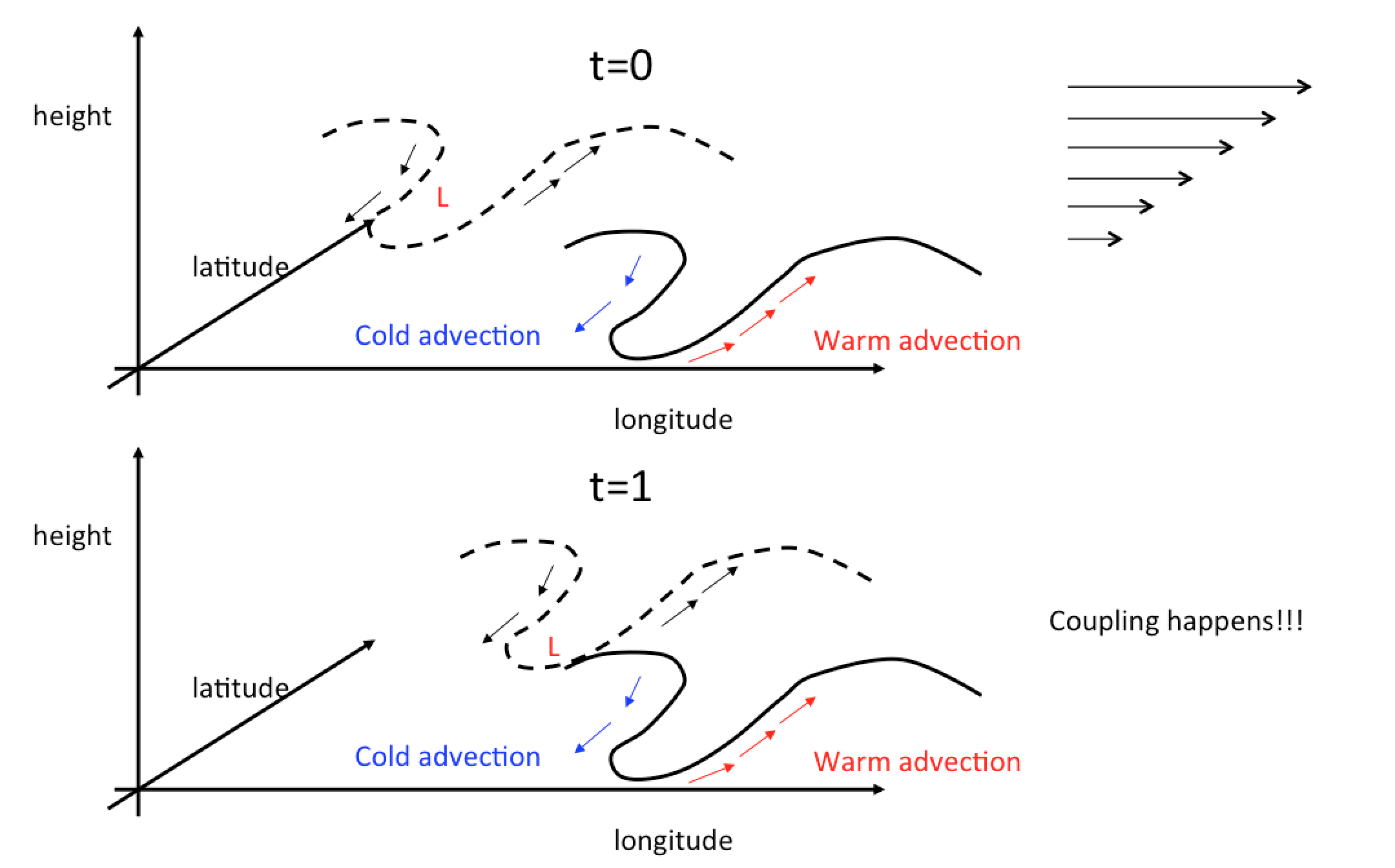
Fig. 4 A schematic diagram showing how the counter-propagating waves over different vertical layers amplify each other. When t=0, the upper-level trough is delayed the lower-level trough by more than 0.25 wave length. However, due to the existence of vertical wind shear, the upper-level trough propagates faster than the lower level trough. In addition, we also know the geopotential height above the near-surface cold advection will decrease with time according to the hydrostatic balance. Thus, when the upper-level trough is spatially collocated with the near surface cold advection, it will be strengthened by the cold advection. This vertical coupling process can increase the amplitude PV, where vertical wind shear and counter-propagating waves are necessary criteria for baroclinic instability.
The other key process for the growth of PV is the barotropic instability. In barotropic instability, the counter-propagating wave happens in meridional direction rather than the vertical direction. Thus, the necessary condition for barotropic instability is the horizontal wind shear. Both barotropic and baroclinic instabilities will lead to the exponential growth of PV anomaly, i.e., \(\frac{Dq'}{Dt}\sim \mathrm{exp}(\sigma t)\), where \(\sigma\) is the growth rate of this system.
Now, some of you might have noticed the connection between (10) and (5). If we linearize the QG-PV equation by assuming \(\mathbf{\bar{u}}\approx U_m\), i.e., the mean flow is dominated by the zonal mean wind, we will find the growth of PV perturbation strongly depends on the existence of wind shear. We will walk through the whole derivation in the homework assignment by using Philips two-layer model.
Note
Here are a few useful physical connections between the first and the second laws of thermodynamics equation, where potential temperature is the key ingredient. From the first law of thermodynamics equation, we know there are two ways to change the internal energy, either through “heat” or “work” (12)
where \(dU=c_v dT\). By adopting \(dP\alpha=Pd\alpha+\alpha dP\) and \(P\alpha=RT\), we can rewrite (12) to
Then, divide the whole equation by \(T\) and adopt the ideal gas law, we can find what left on the l.h.s is entropy \(\dot{Q}/T\) and on the r.h.s. is \(c_pdT/T-RdP/p\), which is the definition of potential temperature. Thus, the conservation of potential temperature is mathematically identical to the conservation of entropy.
From (8) to (9), we can simply use the definition of buoyancy, i.e., \(b'=-\frac{\rho'}{\bar{\rho_0}}g=\frac{\theta'}{\bar{\theta}}g\) and the hydrostatic approximation (i.e., \(b_0=-g\rho_0\) You will need to finish the last step in the homework assignment) to get the hydrostatic thermodynamics equation.
Atmospheric Blocking
A key process that can provide additional predictability is the occurrence of atmospheric blocking. Blocking is a process where the negative PV anomaly cuts off from its adjacent ridge and forms a region with closed PV contour. Different from the elongated feature of trough and ridge, the shape of blocking is relatively round. Due to the inverse cascade of large-scale kinetic energy (more concentrated to the large-scale feature), a round PV is less likely to dissipate until either it is eroded by diabatic process or move back into low PV regions. Thus blocking usually sustains longer than an elongated PV feature.
While blocking is an important predictability source, it is still an unsolved problem. To the best of our knowledge, there are a few processes such as wave activity and teleconnection can change the occurrence frequency of blocking [HMB16]. In numerical experiments, the models with higher spatial resolution tend to simulate more reasonable blocking frequency suggesting the importance of upscale cascade of small-scale wave energy. There are a few interesting mechanisms proposed by Dr. Nakamura at U Chicago, who used a traffic jam model to describe the potential mechanisms of atmospheric blocking. [NH18]
Teleconnections
While the discussion above focuses on the internal dynamics of PV, the external forcing can play important roles for timescales longer than 2 weeks. In equation (9), we omit the external forcing. Thus, the vertical motion-induced adiabatic cooling/warming is always balanced by the horizontal temperature advection. However, with the existence of diabatic term, the balance can change. Here, we provide two different cases to demonstrate how the timescales of external forcing determines the predictability of mid-latitude weather.
In the first case, the characteristic timescales of \(\dot{Q}\) in (8) is much shorter or comparable to the timescales of Rossby wave (14).
In this case, the balance happens within horizontal temperature advection, vertical motion and external forcing. From a climate perspective, the external forcing is dominated by the radiative forcing. Thus, this balance is also called “radiative-advective-convective equilibrium” (RACE). In general, the whole process of RACE (instability adjustment) happens within 2 weeks. For longer timescales, we can only have their equilibrium statistics (i.e., given any two components, we can derive the third).
The second case is that the characteristic timescales of \(\dot{Q}\) in (8) is much longer than the Rossby wave timescales. In this case, the internal dynamics of PV can be considered as a dissipative process, which is always balanced by the external forcing (15) (also see [HK81] for details).
One classic example is the tropical-convection forced tropical-extratropical teleconnection. The large-scale tropical convection such as Madden-Julian oscillation or El Ni~no Southern oscillation (ENSO) can generate large-scale divergence in the upper troposphere. The divergence can perturb the extratropical storm tracks and generate stationary Rossby wave propagating to the extratropical regions. In this case, timescales of forced response is determined by the timescales of forcing rather than the timescales of internal dynamics. Therefore, the predictability of a forced system can be much longer than the one purely determined by the internal dynamics since the external forcings are usually characterized by longer life cycles (e.g., the life cycle of MJO is about 20-90 days and ENSO is about 2-7 years). One prevailing research field is looking for the “forecast opportunity” from subseasonal to longer timescales and the so-called “forecast opportunity” indicates the “external forcing”.
The animation below is an example of tropical-extratropical teleconnection in a barotropic model, where we force the model with a constant divergence forcing (i.e., \(\sigma\sim 0\)). We can find in the later period of integration, the forced response gradually reach a equilibrium state. Similar large-scale patterns can also be found over the extratropical regions if we take the monthly average of 500hPa geopotential height.
Fig. 5 An example of tropical-extratropical teleconnection in a barotropic model. The model is forced by a constant divergence flow (dashed line). The shading shows the vorticity field.
\
Note
Tropical-extratropical teleconection was first discovered by Bjerknes (1969) [Bje69] (although he didn’t spell it out). Then theory was mature around 1980s [HK81], where Sir Brian Hoskins used primitive equation model to investigate the underpinning dynamics. The name of “Rossby wave source” was also established from Sir Brian Hoskins’ work.
References
- Bje69
Jakob Bjerknes. Atmospheric teleconnections from the equatorial pacific. Monthly weather review, 97(3):163–172, 1969.
- HMB16
Stephanie A Henderson, Eric D Maloney, and Elizabeth A Barnes. The influence of the madden–julian oscillation on northern hemisphere winter blocking. Journal of Climate, 29(12):4597–4616, 2016.
- HK81(1,2)
Brian J Hoskins and David J Karoly. The steady linear response of a spherical atmosphere to thermal and orographic forcing. Journal of the Atmospheric Sciences, 38(6):1179–1196, 1981.
- Lor55
Edward N Lorenz. Available potential energy and the maintenance of the general circulation. Tellus, 7(2):157–167, 1955.
- NH18
Noboru Nakamura and Clare SY Huang. Atmospheric blocking as a traffic jam in the jet stream. Science, 361(6397):42–47, 2018.