Week 7: The stability theory¶

In week 6, we learn how to estimate the time evolution of PDF. We can easily find that the analytical solution of LE (i.e., (64)) follows a form of exponential function, where the integral inside the exponent represents the state-dependent error growth rate. For example, if the integral is negative, indicating the volume (density) spanned by ensemble members will increase (decrease) with time at that given location. Thus, it’s pretty much like a stability problem we usually deal with at the traditional geophysical fluid dynamics. For example, in mid-latitude, some regions with strong meridional temperature gradient (vertical wind shear), we can see frontal genesis. These regions have very strong baroclinicity and thus a small disturbance can easily grow. In atmospheric dynamics, we can calculate so-called Eady growth rate, ((74),where $f_0$ is planetary Coriolis Force, $NH$ is Brunt-Vaisala frequency times equivalent depth (i.e., restoring force by buoyancy) and $\Delta U$ is the vertical wind shear) to estimate the environment favoring the baroclinicity.

(74)¶\[\sigma = 0.31\frac{f_0}{NH}\Delta U\]

(74) is a convenient formula for estimating if an environment is bariclinic unstable. However, there are many different kinds of instability and thus a more general framework is required to quantify if an error in initial states will grow with time. In this week, we will introduce three traditional methods (1) Direct method, (2) Energy method, and (3) von Neumann method. All of these methods are widely used in numerical and dynamical system analyses. If any of them indicates instability, the system is either numerically or physically unstable. (One should notice that the system can be physically stable but numerically unstable). Here we use a very simple 1D-advection model to demonstrate how to apply three different methods to analyze the stability in a given system.

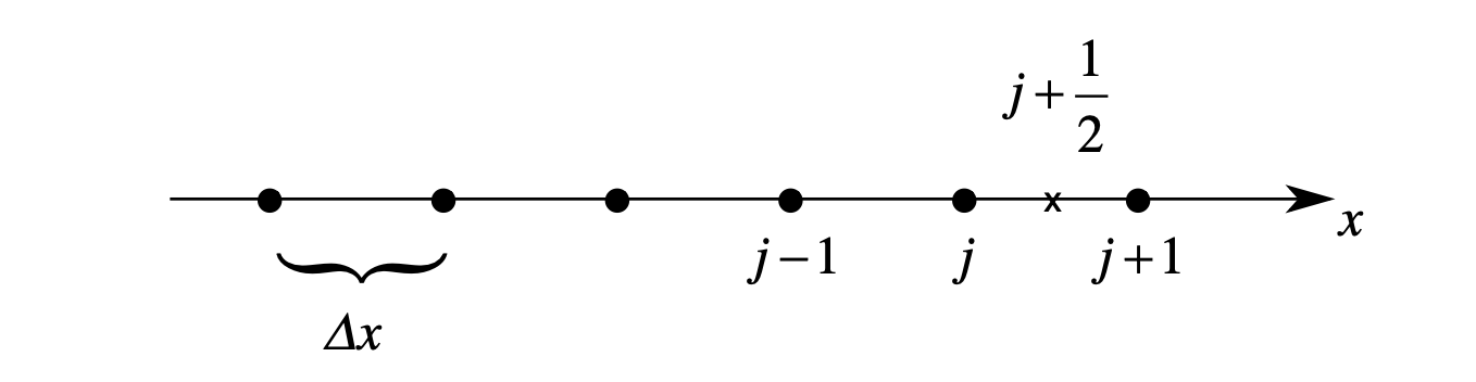
Fig. 15 An example of a one-dimensional grid, with uniform grid spacing $\Delta x$. The grid points are denoted by the integer index j. Half-integer grid points can also be defined, as shown by the x at j+$\frac{1}{2}$.¶

We first start with grid spacing. FIG15 is schematic diagram of 1D grid (sometimes we use mesh or lattice). Since each grid is equally spaced, we can define a function $f(x_j)=f(j\Delta x)$, which further leads to three different definitions of finite difference: (1) For forward difference at point $j$, we have $\frac{f(x_{j+1})-f(x_{j})}{\Delta x}$, (2) for backward difference at point $j$, we have $\frac{f(x_{j})-f(x_{j-1})}{\Delta x}$ and (3) for central difference at point $j$, we have $\frac{f(x_{j+1})-f(x_{j-1})}{\Delta x}$.

Now, we can take a look of the 1D-advection model.

(75)¶\[\frac{\partial A}{\partial t} + c (\frac{\partial A}{\partial x})= 0 \]

with an initial condition

(76)¶\[A(x,0) = F(x) \]

Physically, (75) carries $A_{j}^{n}$ at a position of a particle with a constant speed $c$. We interpret $A_{j}^{n}$ as a conserved property of the particle. To find the analytical solution, we can assume $\xi \equiv x-ct$ and thus $(\frac{\partial x}{\partial t})=c$ (with constant $\xi$). Using the chain rule, we further find that

(77)¶\[\begin{split}\begin{align*} (\frac{\partial A}{\partial x})_{\xi} &= (\frac{\partial A}{\partial x})_t+(\frac{\partial A}{\partial t})(\frac{\partial t}{\partial x}) \\ &= (\frac{\partial A}{\partial x})_t+(\frac{\partial A}{\partial t})(\frac{1}{c}) \\ & = 0 \end{align*}\end{split}\]

and

(78)¶\[\begin{split}\begin{align*} (\frac{\partial A}{\partial t})_{\xi} &= (\frac{\partial A}{\partial t})_x+(\frac{\partial A}{\partial x})(\frac{\partial x}{\partial t}) \\ &= (\frac{\partial A}{\partial t})_x+(\frac{\partial A}{\partial x})c \\ & = 0 \end{align*}\end{split}\]

(77) and (78) suggest that $A$ will conserve as long as it stay on the characteristic line $\xi$. Thus, $\xi$ is an analytical solution of (75) (i.e., $A=f(\xi)$). Now let’s consider using a numerical way to solve (75), which can be written as the form below,

(79)¶\[\frac{A^{n+1}_{j}-A^{n}_{j}}{\Delta t} + c (\frac{A^{n}_{j}-A^{n}_{j-1}}{\Delta x})= 0 \]

Here we use forward difference quotient for time and backward difference for space. We can easily find that what determines the time tendency is the information from upstream (i.e., information is only from one side, i.e., $A_{j-1}^{n}$, and has no dependence on the other side, i.e., $A_{j+1}^{n}$). Let $A(x_j,t_n)$ to be exact solution at the point $t$ and $x$ and $A(j\Delta x, n \Delta t)$ is the numerically solved solution. In general, $A(x_j,t_n) \neq A(j\Delta x, n \Delta t)$ in most cases (but we definitely hope they are the same ;) ). Next, we will examine if (79) is numerically stable.

First, we introduce something called truncation error. For (75), if we use the exact solution $A(x_j,t_n)$, the right hand side of equation will be 0. However, when a discrete form is used, the right hand side of (80) won’t be 0 for most cases i.e.,

(80)¶\[\frac{A^{(n+1)\Delta t}_{j\Delta x}-A^{n\Delta t}_{j\Delta x}}{\Delta t} + c (\frac{A^{n\Delta t}_{j\Delta x}-A^{n\Delta t}_{(j-1)\Delta x}}{\Delta x})= \epsilon \]

and applying Taylor expansion, we know.

(81)¶\[\epsilon = (\frac{1}{2!}\Delta t \frac{\partial^2 A}{\partial t^2}+\ldots)+c(-\frac{1}{2!}\Delta x\frac{\partial ^2 A}{\partial x^2}+\ldots) \]

We say this is a first order scheme given that the $\epsilon$ is a function of second and higher order. To reduce the truncation error, we can select $\Delta x$ as small as possible.

Direct Method¶

In addition to the truncation error which estimates how accurate a numerical differential equation is, we also have discretization error, which estimates how accurate the answer of a differential equation is. However, a decrease in the truncation error does not necessarily ensure a decrease in the discretization error. Discretization error is the difference between the exact solution, $A_{j}^{n}$ and discretized solution $A_{j\Delta x}^{n\Delta t}$. An easy way to visualize the difference between analytical solution and the discretized solutions is using so-called domain of dependence. i.e., plot the discretized solution as a function of $n$ and $j$.

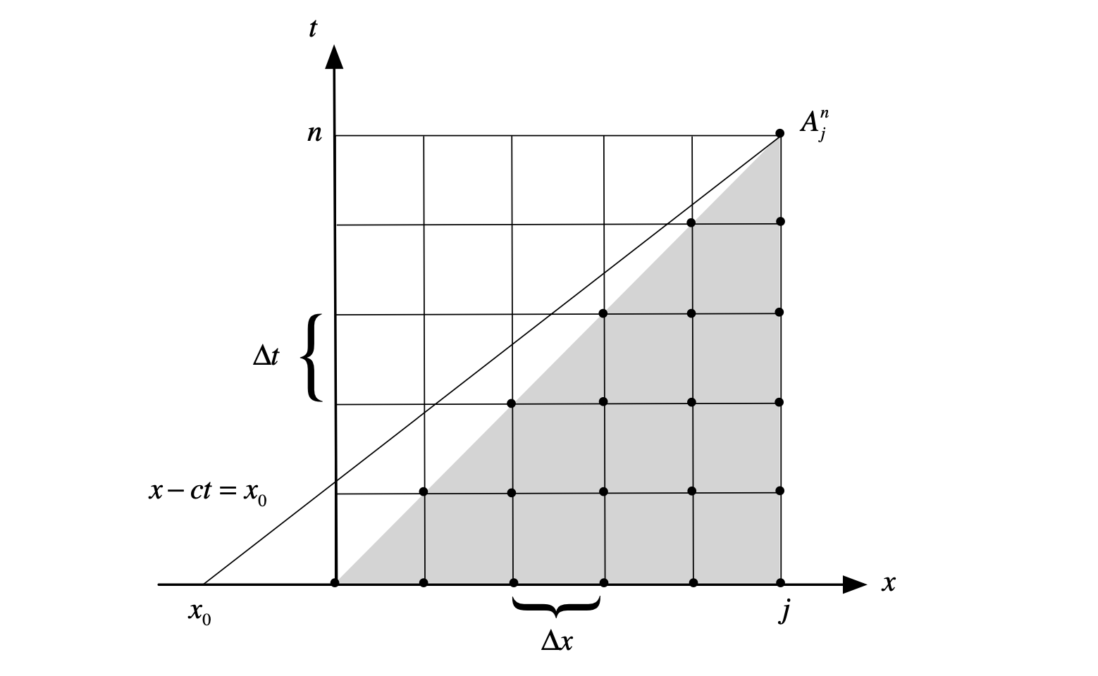
Fig. 16 A schematic diagram of domain dependence. The shading regions show where the “domain of dependence” is for 79. Shading regions are where eq. 79 depends.¶

The shading regions in FIG16 show where the numerical solution should fall in order to get smaller discretization error. If today, the integration starts at a point of $A(x_0,0)$ where $x_0<0$ as indicated by the thin line in FIG16. We can find that the discretization error will never decrease as long as $\frac{\Delta x}{\Delta t$}$ is a constant.

To understand what happens here, we can leverage the analytical solution of (75). For the numerical simulation starts from $A(x_0,0)$, its characteristic line is $\Delta x-c\Delta t=x_0$. Rearranging the equation, it gives us $(1-\frac{x_0}{\Delta x})=c\frac{\Delta t}{\Delta x}$.

(82)¶\[(1-\frac{\Delta t}{\Delta x})=c\frac{\Delta t}{\Delta x}\]

We can easily find, if the discretized solution is identical to the analytical solution, then the second term on the left hand side of (82) will be 0. Therefore, the second term on the left hand side can be considered as the discretization error, which measure the difference between analytical and numerical solutions. In other words, when $c\frac{\Delta t}{\Delta x}=1$, we are certain that $x_0$ is 0. Obviously, $c\frac{\Delta t}{\Delta x}$ is an important parameter for quantifying how close the two solutions (numerical and analytical) are. This parameter is called CFL criteria, named after three great mathematicians: Courant, Friedrichs and Levy.

An alternative way to interpret (82) is through “interpolation and extrapolation”. For example, we can rewrite the upstream scheme as

(83)¶\[A^{n+1}_{j} = (1-\mu) A^{n}_{j} + \mu A^{n}_{j-1}\]

where $\mu$ equals $c\frac{\Delta t}{\Delta x}$. From the schematic diagram below, we can know the solution in the next time step will always be bounded within $A_{j}^{n}$ and $A_{j-1}^{n}$ if $\mu$ is smaller than 1 and bigger than 0. Thus, even in the worst scenario, the signals will be smoothed out rather than exploding.

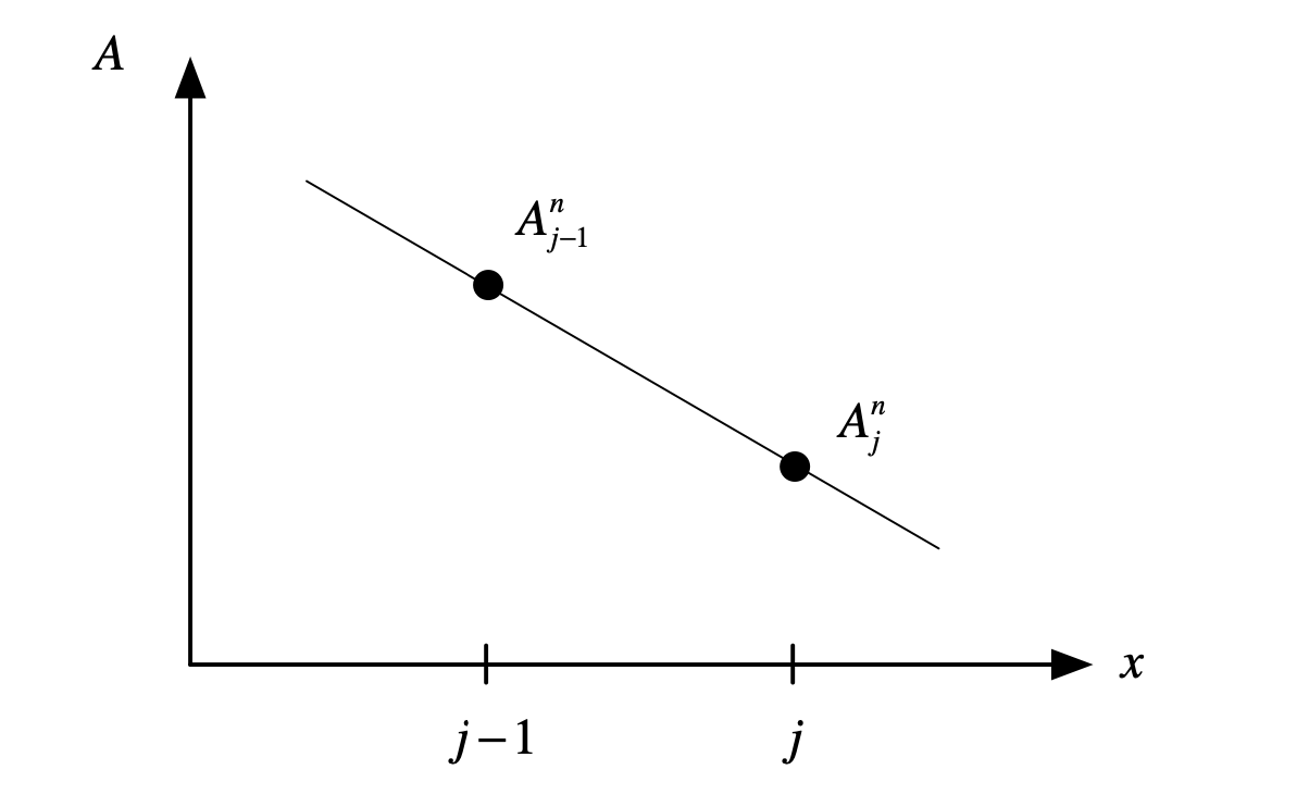
../_images/interprolation_extrapolation.png

Fig. 17 A schematic diagram of “interpolation vs extrapolation”¶

We can rewrite (83) in an absolute form and the following conclusion also holds if $0\geq\mu \geq 1$

(84)¶\[|A^{n+1}_{j}| \leq (1-\mu) |A^{n}_{j}| + \mu |A^{n}_{j-1}|\]

and

(85)¶\[\mathrm{max}_{(j)} |A^{n+1}_{j}| \leq (1-\mu) \mathrm{max}_{(j)}|A^{n}_{j}| + \mu \mathrm{max}_{(j)}|A^{n}_{j-1}|\]

The second line of (85) follows because of $\mathrm{max}|A_{j}^{n}| = \mathrm{max}|A_{j-1}^{n}|$. By inspecting (85), we can again find that the necessary criteria for a numerically stable scheme is

(86)¶\[0\leq \mu \leq 1\]

This approach gives us a direct measurement of the instability in a numerical scheme or any phenomenon of interest. It’s called direct method.

Energy Method¶

The second approach is so-called energy method. Mathematically, we can repeat the same exercise to acquire the same conclusion. I will leave it to the readers to derive the formula. Details can be found in homework instruction.

von Neumann Method¶

In this part, we will walk through another very powerful tool for testing instability, which is called von Neumann method (named after a Hungarian mathematician, John von Neumann). Let’s return to (75) and assume the domain size is infinite for simplicity. This will lead to a wave solution

(87)¶\[A(x,t) = \mathrm{Re}[\hat{A}(t)e^{ikx}]\]

where $|\hat{A}|$ is the wave amplitude. Here we consider a simple wave number for convenience but we can replace the right hand side of (87) with a summation over different wave numbers. Substituting (87) into (75), we have

(88)¶\[\frac{d \hat{A(t)}}{dt} + ikc \hat{A(t)} = 0\]

and the corresponding solution is

(89)¶\[\hat{A}(t) = \hat{A(0)}e^{-ikct} \]

where $\hat{A(0)}$ is the initial states. We can substitute this “time-only” part back to (87) to derive the whole solution (i.e., with both space and time structure).

(90)¶\[A(x,t) = \mathrm{Re}[\hat{A}(0)e^{ikx-ct}]\]

For a finite difference problem, we can assume that the solution has a form of

(91)¶\[A^{n}_{j} = \mathrm{Re}[\hat{A}^{n}e^{ikj\Delta x}]\]

where $\hat{A}^{n}$ is the amplitude of wave $e^{ikj\Delta x}$ at the nth time step. One should notice that $\hat{A}^{n}$ can be an imaginary number, which determines both the phase angle and amplitude of a wave at a given moment.

Now we can define an amplification factor, which measures the growth of $A$.

(92)¶\[\hat{A}^{n+1} \equiv \lambda \hat{A}^{n}\]

For the analytical solution of (75), the amplification factor is $\lambda = e^{ikct}$. This implies that for the exact advection problem with a single wave number, $\lambda = 1$, i.e., the signal won’t amplify or decay.

The question is: what is amplification factor in discrete form? (i.e., numerical solution). For (93), the amplification factor is equivalent to

(93)¶\[\hat{A}(t+\Delta t) \equiv e^{ikc\Delta t}\hat{A}(t) \]

If we start from $t=0$, the numerical solution can be written as a form of amplification factor.

(94)¶\[\hat{A}^{n+1} \equiv \hat{A}^{t=0} \lambda^n\]

therefore, the requirement for model not to blow up is $|\lambda|\leq 1$. To explicitly derive the discrete form of amplification factor, we can substitute (92) back to (79) and have

(95)¶\[\frac{\hat{A}^{n+1}-\hat{A}^{n}}{\Delta t}+(\frac{1-e^{-ik\Delta x}}{\Delta x})c\hat{A}^{n} = 0 \]

we can find that $\hat{A}^{n+1}=(1+\frac{1-e^{-ik\Delta x}\Delta t}{\Delta x})c\hat{A}^{n}$. Comparing with the (88), it is found $\frac{1-e^{-ik\Delta x}}{\Delta x}c$ taking place of $ikc$. To prove this point, we can force $\Delta x \rightarrow 0$ and therefore $\frac{1-e^{-ik\Delta x}}{\Delta x}c \sim ikc$.

If we use the definition of (92) and (95), we can find

(96)¶\[\lambda = 1-\mu (1-\mathrm{cos} k\Delta x+i\mathrm{sin} k\Delta x)\]

where $\mu$ is the CFL. (95) is what we are looking for. However, it’s in a complex form. Thus, we multiply (95) by its complex conjugate to derive the variance of (95).

(97)¶\[|\lambda^{2}| = 1+2\mu(\mu-1)(1-\mathrm{cos(k\Delta x)})\]

Obviously, the amplification factor is also a function of wave number. Physically this make senses because when we say that a signal grows, not only its amplitude but also its phase angle should be considered. For example, when a vector rotates from $[1,0]$ to $[\frac{\sqrt{2}}{2},\frac{\sqrt{2}}{2}]$, the y component increases but the overall amplitude (i.e., $x^{2}+y^{2}$) doesn’t change. Different wave numbers correspond to different rotation rate. We will cover more details in the next section when we talk about the nonmodal system.

Stability in Geophysical Fluid Dynamics¶

The stability theory has been widely applied to different fields. What we learn above is one application in numerical modeling. Here, we leverage barotropic instability for demonstrating how to apply those tools to GFD problems.

Let’s setup our question first. Imagine there is a 2D barotropic flow, which is bounded in meridional direction and periodic in zonal direction. Around the center of domain, we prescribe a background flow (i.e., FIG18), which is positive $\bar{U}$ when $y>L$ and is negative $\bar{U}$ when $y<-L$. In addition, no zonal structure of background flow is given for simplification.

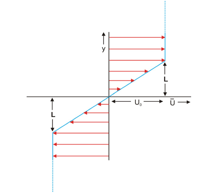
Fig. 18 A schematic diagram of prescribed background flow for shear instability.¶

The corresponding governing equations can be written as:

(98)¶\[\begin{split}\begin{align} \frac{\partial u}{\partial t} +\bar{U}\frac{\partial u}{\partial x}+v\frac{\partial \bar{U}}{\partial y} &= \frac{1}{\rho_0}\frac{\partial p}{\partial x} \\ \frac{\partial v}{\partial t} + \bar{U}\frac{\partial v}{\partial x} &=-\frac{1}{\rho_0}\frac{\partial p}{\partial y} \\ \frac{\partial u}{\partial x}+\frac{\partial v}{\partial y} &= 0 \end{align}\end{split}\]

Consider solutions of the form

(99)¶\[\begin{split}\begin{align} u = \tilde{u}(y)e^{ik(x-ct)} \\ v = \tilde{v}(y)e^{ik(x-ct)} \\ p = \tilde{p}(y)e^{ik(x-ct)} \\ \end{align}\end{split}\]

where c is a complex. Substitute into (98) gives

(100)¶\[\begin{split}\begin{align} ik(\bar{U}-c)\tilde{u}+\bar{U}_y\tilde{v} &= -\alpha_0 ik\tilde{p} \\ ik(\bar{U}-c)\tilde{v} &= -\alpha_0 \tilde{p}_y \\ ik\tilde{u} + \tilde{v}_y & = 0 \end{align}\end{split}\]

by cross-differentiating, we can eliminate $\tilde{p}$ and $\tilde{u}$ and have a single O.D.E. in $\tilde{v}$

(101)¶\[\tilde{v}_{yy}-\tilde{v}(k^2+\frac{\bar{U}_{yy}}{\bar{U}-c}) = 0\]

The general solution for y structure of metidional wind is

(102)¶\[\begin{split}\begin{align} \tilde{v} & = Ae^{-\alpha y} &\; \mathrm{if} \; L\geq y \\ \tilde{v} & = Be^{-\alpha y}+Ce^{\alpha y} &\; \mathrm{if} \; -L\geq y \geq L \\ \tilde{v} & = Fe^{\alpha y} &\; \mathrm{if} \; y\geq -L \end{align}\end{split}\]

Now, we need some boundary conditions to solve A,B, and F in $\tilde{v}$. Consider $\tilde{v}=0$ when $y\rightarrow \pm \infty$. We also need some other conditions to solve the O.D.E. given that the background flow is not differentiable at $y=\pm L$. The first one is the continuity of pressure (because we can dig a hole in fluid). That gives us

(103)¶\[[(\bar{U}-c)\frac{d \tilde{v}}{dy}-\bar{U}_y\tilde{v}]^{y^{+}_{0}}_{y^{-}_{0}} = 0\]

Also, the displace of fluid should be continuous. i.e., $\tilde{v}\equiv\frac{d}{dt}\delta y$ where $\delta y$ is the displacement.

(104)¶\[\begin{split}\begin{align} \tilde{v} & \equiv\frac{d}{dt}\delta y \\ & = (\frac{\partial }{\partial t}+\bar{U}\frac{\partial}{\partial x})\delta y \\ & = (-ikc+ik\bar{U})\delta y \end{align}\end{split}\]

because $\bar{U}$ is continuous over the entire domain and $\delta y$ is continuous, that implies $\tilde{v}$ is also continuous. Thus, (104) will reduce to

(105)¶\[\begin{split}Ae^{-\alpha L}=Be^{-\alpha L}+Ce^{\alpha L} \\ Fe^{-\alpha L}=Be^{\alpha L}+Ce^{-\alpha L}\end{split}\]

Also, apply the jump condition in (104), we can have another two equations

(106)¶\[\begin{split}-\alpha A[(\bar{U}-c)]e^{-\alpha L}=[-\alpha B(\bar{U}-c)-\frac{\partial \bar{U}}{\partial y}]e^{-\alpha L}+[\alpha C(\bar{U}-c)-\frac{\partial \bar{U}}{\partial y}]e^{\alpha L} \\ \alpha F[(\bar{U}-c)]e^{-\alpha L}=[-\alpha B(\bar{U}-c)-\frac{\partial \bar{U}}{\partial y}]e^{\alpha L}+[\alpha C(\bar{U}-c)-\frac{\partial \bar{U}}{\partial y}] e^{-\alpha L} \end{split}\]

Four equations with four unknowns. For nontrivial solution (i.e., $A,B,C,F\neq 0$), we can find the following dispersion relationship.

(107)¶\[(\frac{L\alpha c}{\bar{U}})^2= (L\alpha-1)^{2}-2e^{\alpha L}\]

Ok, after so many steps of derivation, you might wonder where is the stability analysis. If you still remember von Neumann method, we first assume a wave solution and then examine if the solution will grow or not to determine the key parameters. That’s exactly what we are doing for this shear stability analysis!

Similarly, we can apply energy method to derive the necessary criteria for shear stability and I will leave it to readers to derive (hint: multiply (103) by $\tilde{v}'$, which is the complex conjugate of $\tilde{v}$).

Chaos and Predictability

Week 7: The stability theory

Contents

Week 7: The stability theory¶

Direct Method¶

Energy Method¶

von Neumann Method¶

Stability in Geophysical Fluid Dynamics¶