Week 8: The generalized stability theory
Contents
Week 8: The generalized stability theory
In week 7, we learn how to analyze the stability in a numerical scheme and GFD problem. However, there are a few unique cases where the unstable environment doesn’t exist but we still see the growth of unstable mode. You might wonder how is that possible? Atmospheric scientists also found this feature around late 1990s, thus they turned their attention to so-called non-modal system. We will get into more details later; but now, let me quickly recap some concepts we learned over the past few weeks which will be the key ingredients in today’s discussion.
Lyapunov exponent (von Neumann Method in numerical modeling)
Dynamical system
initial uncertainty
We know the weather is intrinsically unpredictable due to the imperfect model physics. However, even in the case where we don’t consider those uncertainties (i.e., the governing equation is deterministic and perfect), we still can’t accurately measure the initial states. Lyapunov exponent is an useful metric for quantifying how the small uncertainties at the initial states grows. Referring back to (3) in week 1 (also (108) here), the variables in a certain dynamical system are specified by finite dimensional state vector \(x\) evolving according to the deterministic equations \(f\).
considering that we initialized the model around the point \(y(t)\) and with sufficiently small error \(\delta y= x\), we can somewhat approximate the model with a linear tangent function.
where \(A(t)\) is the linearized function of \(f(t)\) or so-called Jacobian matrix (if you still remember finding a Jacobian matrix is equivalent to using a linear tangent function to approximate nonlinear dynamics). The matrix \(A(t)\) is usually time dependent and its realizations do not commute in most cases (i.e., \(\mathbf{A(t_1)}\mathbf{A(t_2)}\neq \mathbf{A(t_2)}\mathbf{A(t_1)}\)). Therefore, the error growth cannot be determined from the analysis of the eigenvalues and eigenvectors of \(\mathbf{A(t)}\) because when we swap the order of \(\mathbf{A(t)}\), we can have a totally different matrix. This is so-called non-modal system. The generalized instability theory is developed to solve the non-model problem and focuses on propagator operator, which is a matrix mapping the initial error \(\mathbf{x(0)}\) to the error at time \(t\).
Once \(\mathbf{A(t)}\) is available, \(\Phi (t,0)\) in (110) is readily calculated and can be written as
where \(A(i\tau) = A(t_i)\). If \(\mathbf{A}\) is autonomous (time independent), then the propagator is simply the matrix exponential i.e.,
The deterministic error growth is bounded by the optimal growth over the interval [0,t]
The choice here is based on the absolute amplitude. We can also choose an Euclidean norm, i.e., using the growth of total variance/energy to define the growth of signals \(||\mathbf{x(t)}||^2\).
If we choose an Euclidean norm, (113) can be written as,
where \(\mathbf{\Phi (t,0)}^{T}\mathbf{\Phi (t,0)}\) indicates how much the signals have amplified. For (114), if we can find a matrix, \(v\), which gives us \([e^{\mathbf{A}t}]^{T}[e^{\mathbf{A}t}]v_i = \lambda_iv_i\), where \(\lambda_i\) is a constant, then (114) will reduce to
We also know that \(\mathbf{\Phi (t,0)}^T\mathbf{\Phi (t,0)} = e^{2At}\). Thus, (115) is equivalent to finding the eigen value of \(A\) (i.e., \(\lambda_{A,i}\), which is a diagonal matrix) and calculating the exponential of \(\lambda_{A,i}\) matrix. The real part of \(\lambda_{A,i}\) represents growth rate and the imaginary part represents the oscillatory component. This is in general consistent with the traditional stability analysis (von Neumann method).
Modal vs non-modal
One key ingredient in generalized stability theory is non-modal system. Physically, modal is defined as that eigen vectors of \(x^Tx\)(or EOF mode in climate science) capture all necessary dynamics regardless of time. However, modal dynamics can’t capture the transient growth of the error, which is important for weather prediction and initiation of the low-frequency variability (so-called stochastic forcing).
To demonstrate the difference between modal and non-modal system, we repeat the same exercise in (115) but apply the eigen value decomposition to A instead this time
\(\lambda_{A}\) is an diagonal matrix, which contains the eigen value of \(A\) along the diagonal direction and \(S\) is the eigen vector. In general, \(\lambda_{A}\) is negative in its real part and is arranged in an order from the largest to the smallest (slow- to fast-decaying mode). A negative \(\lambda_{A}\) indicating the memory from initial states will gradually decay with the increase of forecast lead time.
Given a small t (because we are focusing the transient time scales), we know \(e^{2S\lambda_{A}S^{-1}t}=||S e^{\lambda_{A}t}S^{-1}||^{2} \leq ||S||^2||S^{-1}||^2 e^{2\lambda_{A}t}\leq ||S||^2||S^{-1}||^2 e^{2\lambda_{A,\mathrm{max}}t}\) . Thus, \(||S||^2||S^{-1}||^2 \) determines the upper-bound of \(e^{2S\lambda_{A}S^{-1}t}\). For the lower bound, we know \(e^{2\lambda_{A,min}t} \leq e^{2At}\), i.e., \(e^{2At}\) cannot decay faster than the fastest decaying mode. Combining both condition gives us:
if \(||S||^2||S^{-1}||^2 = 1\) and \(\lambda_{A,max}=\lambda_{A,min}\), suggests that all three terms in the inequality of (117) are the same and the dynamics of \(f\) is governed by the mode dynamics (linearly stable) and there is no significant difference between any two unstable mode. In this case, we can consider that all of the eigen modes have reached a statistical equilibrium state and their transient interaction doesn’t influence the dynamics of interest. This is the case when we talk about how the weather signals are represented in a climate change problem. Because in a climate change time scales (>10 yrs), all the weather signals have already reached an equilibrium states.
However, this is not the case when the time scales of interest is much shorter i.e., hourly to seasonal time scales. In these time scales, \(||S||^2||S^{-1}||^2 e^{2\lambda_{A,\mathrm{max}}t} >> 1\) indicates we can still observe some instability caused by non-modal process. For example, if today we have two eigen modes, \(\phi_1\) and \(\phi_2\). The phenomenon of interest is their linear combination, let say \(\phi_1-\phi_2\). Given the fact that \(\phi_1\) decays much slower than \(\phi_2\), we can find that the amplitude of \(\phi_1-\phi_2\) grows with time even both \(\phi_1\) and \(\phi_2\) are getting smaller and smaller. (see FIG19)
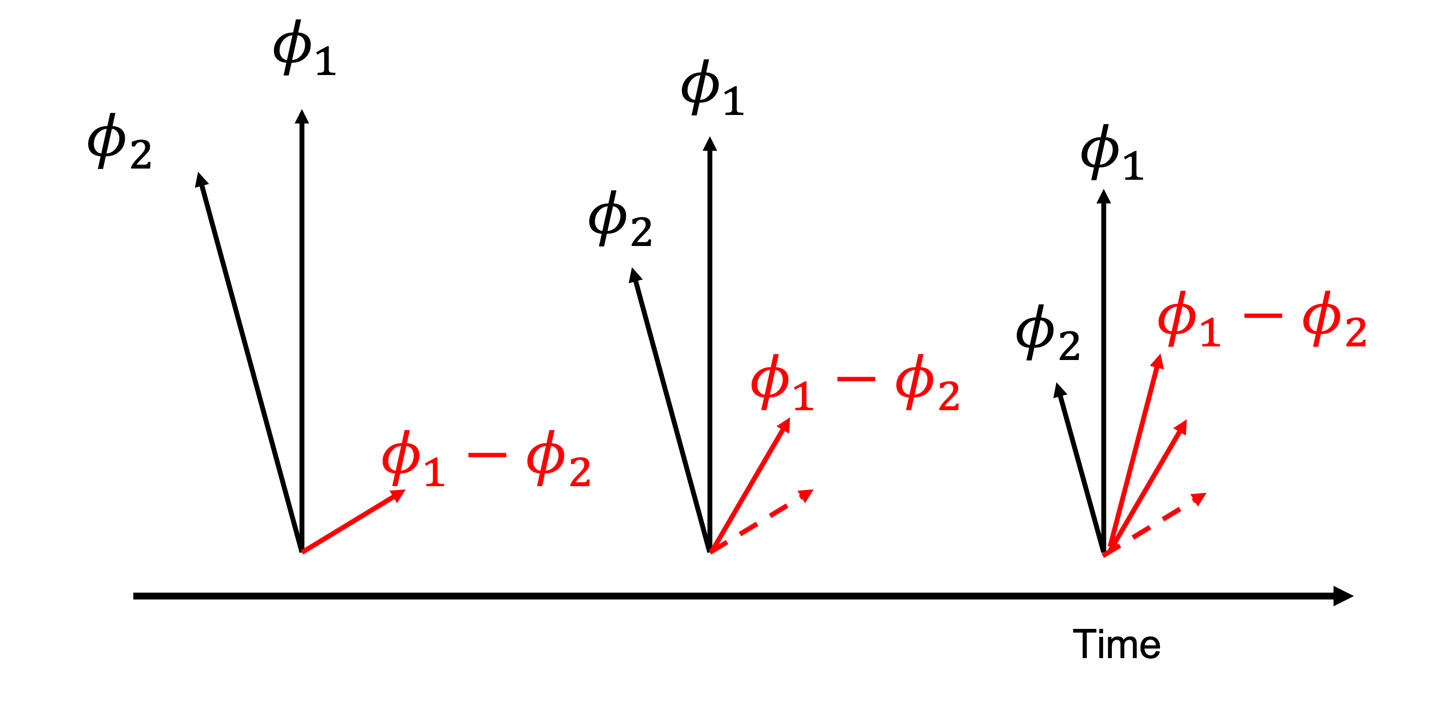
Fig. 19 An example of non-modal growth of signals at finite time.
The question is what kind of phenomenon is most likely to experience non-modal growth. From (117), we know that the eigen vector \(v_i\), who has the largest \(\lambda\), will experience the most significant error growth. One should notice that the \(v_i\) is different from the eigen modes of state vector. The former quantifies the most unstable signal/initial state while the later quantifies the mode which explains the most variance. There is one unique case that these two are identical, I will let the readers think about what is that? (HW).
Examples of generalized stability problem
Case I
Here we use two examples to demonstrate the finite amplitude of error growth lead by the non-modal dynamics.
where \(A\) is autonomous. In this case, we can find the diagonal elements are 0.9 indicating that \(A\) is negative and the signal will decay with the increase of forecast lead. However, if we we choose the right initial state, the initial error can still experience significant growth.
In the following figure, we plot the ratio of variance (\(||e^{2At}||\)) between the initial and the final states as a function of time. Blue curve shows the most unstable case and the red curve shows the result when \([1,0]\) is used as the initial state.
#s = np.random.normal(0, 0.1, 1000)
dim      = 100
growth1  = np.zeros((dim,1))
growth2  = np.zeros((dim,1))
a        = np.array([[0.9,0.3],[0.,0.9]])
x_0      = np.array([[1],[0]])
for tau in range(0,dim):
    G_tau    = np.linalg.matrix_power(a, tau)
    x_tau    = np.matmul(G_tau,x_0)
    h        = np.matmul(np.matrix(G_tau).getH(),G_tau)
    w,v      = np.linalg.eig(h)
    growth1[tau,:] = np.max(w)
    growth2[tau,:] = np.matmul(np.transpose(x_tau),x_tau)/np.matmul(np.transpose(x_0),x_0)

plt.figure()
plt.plot(growth1,'b', label='Nonmodal')
plt.plot(growth2,'r', label='Modal')
plt.legend()
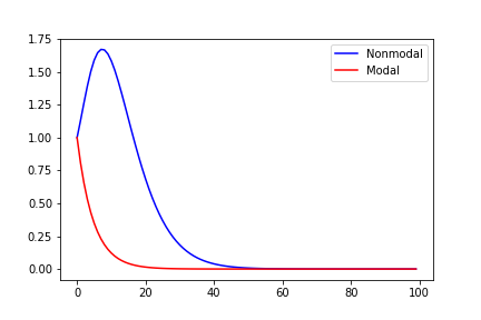
Fig. 20 The error growth in the optimal case (blue) and using [1,0] as initial state (red)
In FIG20, we can find that both blue and red curves gradually decay to 0 when t is big enough. However, the blue curve shows transient growth when \(t=15\).
Case II
I the second case, we choose two stable linear operators (119) but we swap them regularly.
where \(\omega_1 = 1/2\) and \(\omega_1 = 3\). In the case where there is only one operator, the system trajectory lies on a constant energy surface. However, if we swap the linear operator for every \(T=\frac{\pi}{2\omega_1}\) and \(T=\frac{\pi}{2\omega_2}\), we can find the amplitude grows exponentially.
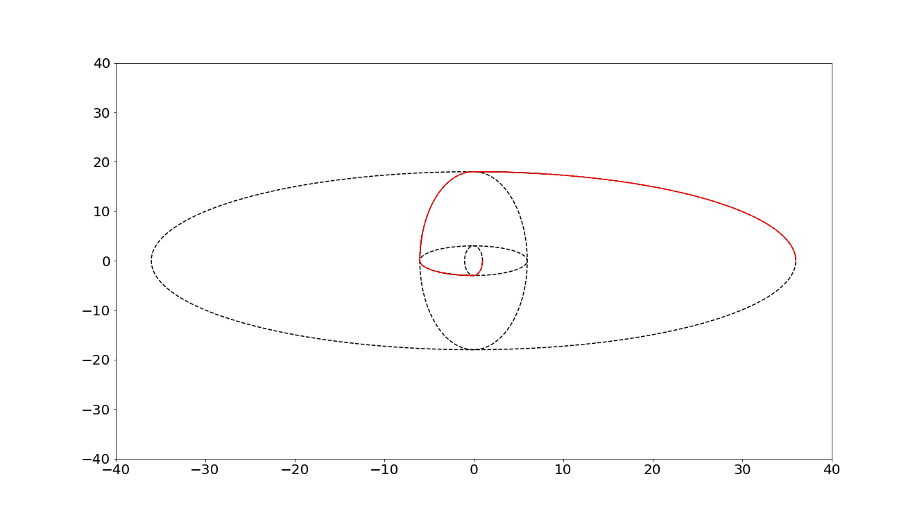
Fig. 21 Red curve shows the case where we swap the linear operators for every quarter period.
This feature has very important applications. In mid-latitude regions, the environment is usually not baroclinicly unstable. However, we still observe many baroclinic waves. [] (also see Ch5 in [PH06]) provides a very clean explanation. According to week 2, we know that one necessary criteria of baroclinic instability is the change of sign in background PV gradient. This can lead to counter-propagating baroclinic Rossby wave. However, in an environment where PV gradient never change sign, can we still have counter-propagating wave? The answer is yes.
Similar to FIG19, if there are two modes to construct a barolcinic wave. One decays faster and has shorter period than the other. Their linear combination can lead to the transient growth of the wave signals. If the transient growth over different \(t\) can be accumulated, we can see asymptotically unstable waves.
def f(L,y):
    return np.matmul(L,y)

# define RK4
def rk4(L,t0,y0,tn,n):

    # Calculating step size
    h = (tn-t0)/n

    #print('\n--------SOLUTION--------')
    #print('-------------------------')
    #print('x0\ty0\tyn')
    #print('-------------------------')
    for i in range(n):
        k1 = h * (f(L,y0))
        k2 = h * (f(L,(y0+k1/2)))
        k3 = h * (f(L,(y0+k2/2)))
        k4 = h * (f(L,(y0+k3)))
        k = (k1+2*k2+2*k3+k4)/6
        yn = y0 + k
        #print('%.4f\t%.4f\t%.4f'% (x0,y0,yn) )
        #print('-------------------------')
        y0 = yn
        #print(y0)
        t0 = t0+h
    return yn

# see Ch5 of Palmer and Hagedorn 2008 for more details: https://www.cambridge.org/core/books/predictability-of-weather-and-climate/9A8E7E0A16BC8BA928243F46ED192FE6
# using RK4 for numerical integration
omega1  = 3
omega2  = 0.5
A1      = np.array([[0,1],[-omega1**2,0]])
A2      = np.array([[0,1],[-omega2**2,0]])
v       = np.array([[1],[0]])
record  = np.zeros((1000,2))
record[0,:] = np.reshape(v,[2,])
record2 = np.zeros((10,1000,2))
t       = 0
count   = 0
for i in range(10):
    # swapping linear operator for every quarterly period
    if (i % 4) == 0:
      A=A1
      omega=omega1
    elif (i % 4) == 1:
      A=A2
      omega=omega2
    elif (i % 4) == 2:
      A=A1
      omega=omega1
    elif (i % 4) == 3:
      A=A2
      omega=omega2
    v_template       = v
    for j in range(999): # fixed operator
        t_index          = np.linspace(0,20,1000)
        v_new            = rk4(A,t_index[j],v_template,t_index[j+1],100)
        record2[i,j,:]   = np.reshape(v_new,[2,])
        v_template       = v_new
    for j in range(100): # swapping linear operators
        t_index         = np.linspace(0,np.pi/(2*omega),101)
        v_new           = rk4(A,t_index[j],v,t_index[j+1],100)
        record[count,:] = np.reshape(v_new,[2,])
        count           = count+1
        v               = v_new


fig=plt.figure()
plt.plot(record2[0,0:110,0],record2[0,0:110,1],'k--')
plt.plot(record2[1,0:700,0],record2[1,0:700,1],'k--')
plt.plot(record2[2,0:110,0],record2[2,0:110,1],'k--')
plt.plot(record2[3,0:650,0],record2[3,0:650,1],'k--')
plt.plot(record[0:400,0],record[0:400,1],'r')
plt.xlim([-40,40])
plt.ylim([-40,40])
plt.xticks(fontsize=20)
plt.yticks(fontsize=20)
fig.set_size_inches(18.5, 10.5)