Week 5 and 6: Laplace Transform#
What is a Laplace Transform and how it works? (s space and t or x space)#
From the first two chapters, we know a lot of ODEs share a similar form of solution : i.e., \(c_1e^{s_1t}+c_2e^{s_2t}\). When we substitute the solution back to the ODEs, we can usually subtract the exponential term and make the entire equation into an algebra problem. This is exactly the goal of Laplace Transform, which can be simplified as the flowchart below.
From the flowchart, we can find the role of Laplace Transform is converting the entire equation from t space to the s space and simplify the problem. Mathematically, it can written as
One can consider (62) as a projection or mapping of \(f(t)\) onto the s space.
Example 6
Let \(f(t)=e^{at}\), with a non-zero a. The Laplace Transform of \(f(t)\) is
The Laplace Transform exist when \((a-s)<0\), which will lead to
One should notice that \((a-s)<0\) is the necessary criteria for the existence of Laplace Transform of a function. That also means, if any function which has a growth rate \(a\) greater than \(s\), then there is no Laplace Transform of that given function. A very famous example is the function \(e^{t^2}\), which doesn’t have a Laplace Transform.
Table 1 are some of the widely used Laplace Transforms. Readers can follow the example above to find the Laplace Transform of the corresponding function.
Table 1
One can find that Laplace Transform is linear, indicating any rules applied to a linear operator is also applied to Laplace Transform. i.e., \(\mathcal{L}(f(x)+g(x))=\mathcal{L}(f)+\mathcal{L}(g)\) and \(\mathcal{L}(af(x))=a\mathcal{L}(f(x))\).
For the inverse transform, we can setup a problem, where we would like to find a function leads to
One should notice that \(\mathcal{L}^{-1}\) needs to be a function of \(s\) since we would like to transform \(F(s)\) back to \(t\) space. By observing (63), we can find it with a form of
If readers still recall the complex roots of a constant coefficient ODE, it usually shares a solution of \(e^{\alpha t}\cos(\beta t)+e^{\alpha t}\sin(\beta t)\). The \(\alpha\) in the upper/lower bound of the integral is identical to the meaning of \(e^{\alpha t}\), where we specify a basis for projection should have a certain growth rate \(\alpha\). On the other hand, \(-i\infty\) and \(i\infty\) indicates we loop over all possible wave number \(\beta\), because sometimes we can have multiple \(\beta\). Readers can find the proof of inverse Laplace Transform here. We will cover more details in the chapter of Fourier Transform. ((63) and (64) are actually a more general definition of Fourier and inverse Fourier Transforms.
Initial Value Problem#
To deal with an initial value problem, we first need to know the Laplace transform of a derivative. i.e.,
Using integrate by part, we can find
Similarly, we can go to higher order derivative
It is evident that if we would like to calculate the Laplace Transform of the 2nd-order derivative, we need the initial condition from the 0th-order and the 1st-order, which is consistent with what we learn in week 1.
The readers can try to go to higher order derivative. It can be proofed that
Example 1
Solve the following ODE with Laplace Transform
As we know \(\mathcal{L}[y'] = sY(s)-y(0)\), \(\mathcal{L}[y] = Y(s)\) and \(\mathcal{L}[1] = \frac{1}{s}\). This leads to
Rearrange the above equation,
From the table above, we know
(Readers can use integrating factor to have the same answer).
Example 2
Solve \(y^{''}+4y^{'}+3y=e^{t}; \; y(0)=0; \; y^{'}(0)=2\)
First, we take Laplace Transform of each term
which yields
or
reorganize the equation, we can have
From the table above, we know
(hint: Readers can solve this problem by using undetermined coefficients)
Heaviside Function and Shifting Theorem#
Laplace Transform is a unique way of solving an initial value ODE. What it provides that previous methods do not, is its ability of handling discontinuity. i.e., piecewise continuous.
First, let’s define what is a piecewise continuity. It can be any of the following three conditions.
Piecewise Continuity
(1) \(f\) is continuous at all but perhaps finitely many points of \([a,b]\)
(2) if \(f\) is not continuous, then \(f(t)\) has a finite limits as t approaches \(t_0\) from the left and from the right.
(3) \(f(t)\) has a finite limit as t approaches a from the right and also t approaches b from the left.
Mathematically, this discontinuity can arise from filtering the data. In a real-world case, the localized SST forcing or convection can yield similar effects. One of the impulse forcing experiments, which has been widely used in atmospheric science, is called Green’s function approach. Dr. Yen-Ting Hwang in our department is an expert in this field. On the hand, when we study how the convection over the hurricane eyewall drive the transverse circulation, we use similar approach to handle the problem (more details will be covered in the Chapter of special function).
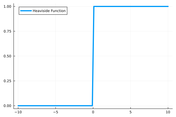
To know the connection between impulse and Laplace Transform, we will walk through two shifting theorems first. We will start with the second shifting theorem of Laplace Transform since it’s physically more intuitive. Inspecting (62), we can already find the condition for discontinuity in Laplace Transform. The lower bound of the integral starts from 0, indicating any \(f(t)\) with \(s<0\) is discarded. We can consider function \(f(t)\) is multiplied by a unit step, i.e., Heaviside function, which is defined as
From the figure below, we can see that Heaviside function acts as an filter.

Fig. 3 A schematic of Heaviside function with a jump condition at \(t=0\)#
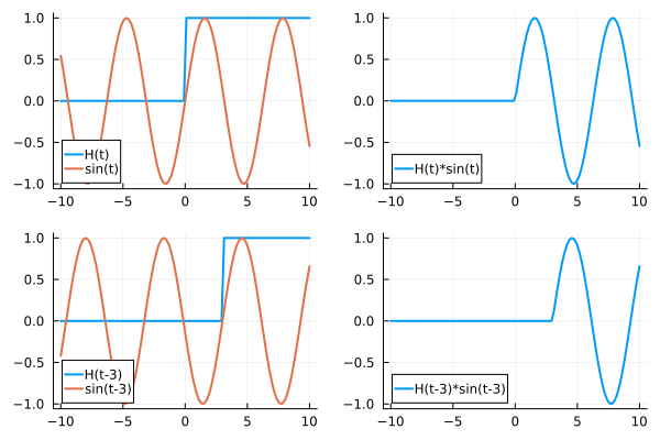
Now we can picture a new function, where we shift both \(f(t)\) (the function which we would like to apply an Laplace Transform to) and Heaviside function slightly to the right…let’s say by 3. Using a \(\sin(t)\) as an example, the figure below shows the function before (upper panel) and after the shifting (lower panel).

Fig. 4 The second shifting theorem#
We can find the entire function remains the same shape. If we take the Laplace Transform of the function above,
Here we define a new t coordinate, \(t_{\textrm{new}}\), where \(t_{\textrm{new}}=t-3\), and use it to rewrite (70)
Example 3
Determine the Laplace Transform of
We can first observe where the discontinuity happens. According the jump condition above, we know it happens at \(t=2\). Therefore, we can define a new \(t_{\textrm{new}}=t-2\) and rewrite the equation.
or
Then we can take Laplace Transform for the equation above, which gives us
Now let’s look at a real ODE problem.
Example 4
Consider
where
Before we dive right in, readers can think about what methods other than Laplace Transform can be applied to this problem. By observing the equation, we can find it can solved by constant coefficient method plus the undetermined coefficients. It is evident that the general solution would be something like,
Now let’s define a new coordinate \(t_{\textrm{new}}=t-3\). This enables us to rewrite the equation
and
Using Laplace Transform,
Rearrange the equation,
Assume we can decompose the equation above into different linear components
(There is a small tip, when we apply such decomposition, we can set the numerator has an order small than the denominator.)
We will find \(A=\frac{3}{4}\), \(B=\frac{1}{4}\), \(C=-\frac{3}{4}\), and \(D=-\frac{1}{4}\) i.e.,
Take the inverse Transform will lead to the final form of solution
and
which is consistent with our first guess based on constant coefficient + undetermined coefficient methods.
In addition to the shift of function over the t space, we can also shift it over the s space (complex space), which is the first shifting theorem. Inspecting (62), we can find to shift a function on s space, we need a function of \(e^{at}\).
If we multiply the original function \(f(t)\) by \(e^{at}\) and take the Laplace Transform,
we can see the function was shifted by a in s space.
From equations (72) and (71), one can find some similarity between the first and the second shifting theorems.
If we would like to shift a function over physical space (t space), we need to multiply its Laplace transform (s space counterpart) by \(e^{-as}\). Similarly, if we would like to shift a function over complex space (s space), we need to multiply the function at the physical space by \(e^{at}\).
Example 5
Determine
we can first organize the function into a form of \(e^{at}f(t)\). Let \(s_{\textrm{new}}=s+2\)
Convolution#
Another widely used technique in atmospheric science, signal processing, and machine learning is called convolution. In atmospheric science, it has another famous nickname: running average or running mean.
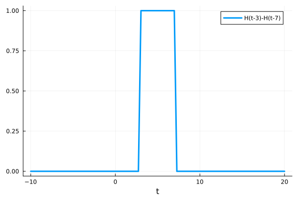
We can start from (69). Here we take the difference of two Heaviside function \(H(t-a)\) and \(H(t-b)\) with \(b>a\). This will create two jump conditions:
(73) is visualized in the figure below.

Fig. 5 A schematic of Heaviside function with two jump conditions at \(t=3\) and \(t=7\)#
Now we introduce a new operator, convolution Mathematically, it is written as
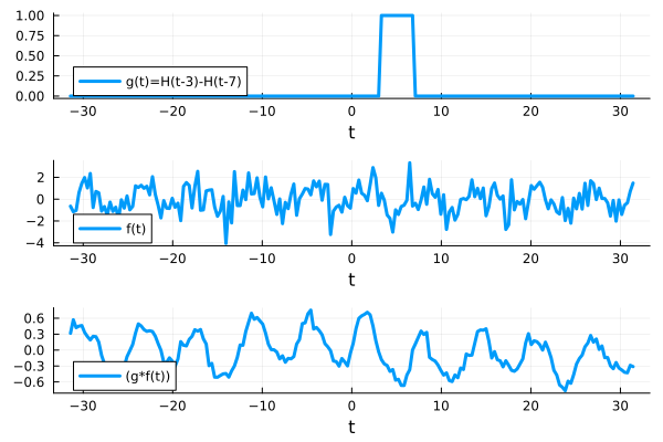
(74) indicates if we first divide \(f(t)\) into infinite data points \(f(t_i)\) and take the average for the first data point from \(t_1-\frac{b-a}{2}\) to \(t_1+\frac{b-a}{2}\). After the calculation, we repeat it all over again for \(t_2\) and so and so forth until we loop over the entire \(f(t)\). This can be visualized with the figure below.

Fig. 6 A schematic of how convolution works when we apply a Heaviside function with a window size of 4 to a noisy data. (top): The Heaviside function used for calculation (middle): the raw time series, \(f(t)\), and (bottom): \((g*f)(t)\)#
From the figure above, one can find that \((f*g)(t)\) has less wiggles than the original time series \(f(x)\) indicating when we apply a mask with a constant value for convolution, it can smooth out the high frequency noise. We can also have different shape of \(g(t)\) for convolution. (see later examples)
There are some very important characteristics for the Laplace Transform of a convolution, so-called convolution theorem.
and
(75) tells us the Laplace Transform of convolution of two functions equals the multiplication of each other’s transforms. so does the inverse transform.
Example 6
Find
From the convolution theorem, we can assume
where
then
Example 7
Find the solution of
Take the Laplace transform of both sides of the equation, we have
and solve for \(Y(s)\)
fractionalize \(Y(s)\), we have
Apply with the inverse transform,
Readers can substitute \(f(t)\) with any function of interest to get the final solution.
Impulse, Dirac Delta Function and Green’s Function approach#
Following (73), if one makes the gap between \(a\) and \(b\) extremely small, let’s say nearly 0. Then, the window in (73) will become an impulse. Here we define a function, Dirac Delta Function.
when the duration goes to \(0\), the height of shock goes to infinity. The Laplace transform of the Dirac Delta function also has a very special quantity. For example, if today we have a shifted pulse,
and take the Laplace transform,
if we don’t have any shift, \(\mathcal{L}[\delta_{\epsilon}(t)](s) = 1\).
Example 8
Find the solution for the following
Applying Laplace Transform to the differential equation, we have
Reorganize the equation,
Then
if we focus on \(\frac{1}{(s+1)^2+1}\) first and leverage the first shifting theorem
then substitute \(e^{-3s}\) back to the equation and use the second shifting theorem, we can have the final form of solution
