Week 9 and 10: Special Functions#
Special Functions, Series Solutions and Recurrence Relations#
Following the discussion of Sturm-Liouville form in the last chapter, we will go a step further to check the cases of \(r(x)\neq 1\), \(q(x)\neq 0\), and \(p(x)\neq 0\). Indicating that we have inhomogeneous grid spacing. Some cases such as cylindrical coordinate, spherical harmonics and parabolic cylinder functions, all of their solutions correspond to a set of Sturm-Liouville equation with \(r(x)\neq 1\), \(q(x)\neq 0\), and \(p(x)\neq 0\). The reason why these special functions are important is that they have been widely used in geophysical fluid dynamics, quantum physics and electromagnetism. To solve these special functions, series solutions play the most important role where we will leverage it for finding the recurrence relation of each special function.
Bessel Function#
The origins and solutions#
Bessel function is the solution of Laplace equation on cylindrical coordinate. (see figure below). Considering a diffusion equation on a cylindrical coordinate,

Fig. 10 Cylindrical coordinate.#
(94) is a partial differential equation. While we will cover more details in the later chapter, let us assume that (94) can be simplified by introducing separation of variables. i.e.,
where \(X(x)\), \(\Phi(\phi)\) and \(Z(z)\) are radial, tangential and vertical structure of the solution.
By substituting (95) into equation (94), we can have
where \(k\) and \(\mu\) are eigen values for vertical and tangential solutions respectively. Here, we focus on the radial structure given that the vertical and tangential solutions can be solved using Fourier series.
By rearranging (96), we can have
Observing (97), one can find that this problem can be solved by combining Euler form with series solutions (we usually assume the solution has a form of \(e^{At}\)). By assuming the solution has a form of
which gives us
and
Substituting (98), (99), and (100) into (97), we can find
or
To get a non-trivial solution, we need \([r(r-1)+r-\nu^2]=0\), and \([[(n+r)(n+r-1)+(n+r)-\nu^2]c_n+c_{n-2}]=0\). (reader can think why we don’t give the same constraint to \([(r+1)(r)+(r+1)-\nu^2]\)). This forms a complete set a recurrence relationship. i.e.,
from the first equation, we know \(r\pm \nu\). This also gives us \(c_1=0\) according to the second equation of (103). Similarly, solving for \(c_n\), we have a recurrence for \(n\geq2\)
On the other hand, because \(c_1=0\), we have
according to (105), we can find the entire equation is an even-indexed function (any odd-indexed term is dropped). This also indicates we can define a new index, \(n=2N\), to rewrite (104).
based on (106), we can find the relation between \(2N\)th-order term with the \(0\)th-order term. i.e.,
Therefore, the solution of Bessel function can be written as
This is a nontrivial solution of Bessel function of order \(\nu\) for any nonzero choice of constant \(c_0\). This solution is usually expressed expressed in terms of the gamma function, which is defined as
One can find that it looks very similar to the Laplace Transform of \(t^{x-1}\) indicating that we can solve the problem using integrate by part.
The term \(-t^{x-1}e^{-t}|_{t=0}^{t=\infty}\) is apparently 0, suggesting
If we go all the way to \(\Gamma(1)\)
and given the fact \(\Gamma(1)=1\), we find \(\Gamma(x)=(x-1)!\). Similarly, one can prove \(\Gamma(x+\nu+1) = (x+\nu)\cdots(3+\nu)(2+\nu)(1+\nu)\Gamma(\nu+1)\). Substitute this relation back to (108), we have
for homogeneous problem, \(c_0\) can be an arbitrary (but nonzero) constant. If we choose, \(c_0=\frac{1}{2^{\nu}\Gamma(1+\nu)}\), then the entire equation can be written as
(114) is so-called Bessel function of the first kind of order \(\nu\)
But don’t forget, the Bessel function is a 2nd-order ODE. This indicates we have another set of solution which is linearly independent of (114). One such solution is the Bessel function of the second kind of order \(\nu\) (also known as Weber function), which is denoted \(Y_{\nu}\). It’s related to the first kind as follows:
where \(J_{-N}=(-1)^{N}J_{N}\) (readers can try to prove this equation by assuming \(N_{\textrm{new}}=N-\nu\)). An alternative form of (115) to represent the second kind of Bessel function solution with \(\nu=0\) is
where \(\phi(n)=1+\frac{1}{2}+\frac{1}{3}+\cdots+\frac{1}{n}\) and \(\gamma=\lim_{n\rightarrow\infty}(\phi-\ln(x))\sim 0.57721566\cdots\)
Back to (115), when \(\nu\rightarrow N\) (N is an integer), readers can find the following relation according to L’Hôpital’s rule (I will leave this practice to readers).
Notes
To prove that \(Y_{\pm\nu}=\lim _{\nu\rightarrow N} [\frac{\partial J_{\nu}}{\partial \nu}-(-1)^N\frac{\partial J_{-\nu}}{\partial \nu}]\) is a solution of Bessel function, we can take the derivative of the second equation of (97) with respect to \(\nu\)
we have
if we let \(X=J_{\nu}-(-1)^N J_{-\nu}\), we can find \(\frac{\partial}{\partial \nu}J_{\pm\nu}\) is the solution of Bessel function if and only if \(2\nu X \rightarrow 0\). It’s not hard to find \(J_{\pm\nu}=0\), given \((-1)^NJ_{-\nu}= (-1)^{2N}J_{\nu}=J_{\nu}\).
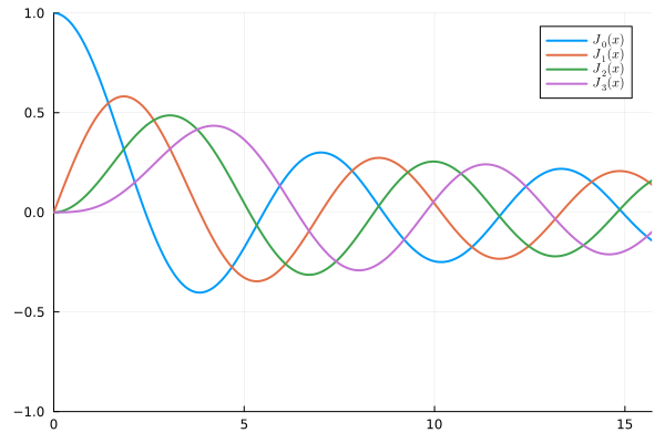
Based on (114), we can plot the solution of Bessel function of the first kind with different \(\nu\).
using Plots
using SpecialFunctions

x  = range(0.001, 5π, length=1000)
bessel_output = zeros(Float64, 5, 1000)
for nu  in 0:4
    sum_x = zero.(x)
    for j in 0:100
        sum_x = (-1).^j*1/(gamma(j+1)*gamma(j+nu+1))*(x/2).^(2*j+nu)+sum_x
    end
    bessel_output[nu+1,:] = sum_x
end

Fig. 11 An visualization of Bessel function solution of the first kind with \(\nu=0-4\)#
The readers can also try to plot Bessel function solution of the second kind and visualize the result.
Modified Bessel function#
There is one special kind of Bessel function where the coordinate is defined on imaginary coordinate i.e., \(x=ix\). If we use \(ix\) to replace \(x\) (or \(k\)=\(ik\)) in the first equation of (96), we can have so-called modified Bessel function.
Modified Bessel function is a more widely used form in atmospheric science, where the wavy solution in radial direction (i.e., along \(x\)) becomes an exponent-like function where the solution is one-side bounded. i.e., \(X=0\) when \(x=0\) or \(x=\infty\). On the other hand, the exponent-like function in \(z\) direction becomes a Fourier-series problem (i.e., Sturm-Liouville with \(p(x)=1\)). In atmospheric science, it is called vertical normal mode decomposition.
The first kind of solution of the modified Bessel function is related to the original Bessel function as follows:
and so is the second kind
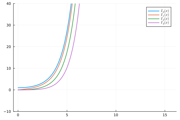
The figure below visualizes the first kind solution of the modified Bessel function.

Fig. 12 An visualization of modified Bessel function solution of the first kind with \(\nu=0-4\)#
One can easily find the solution is bounded on one end but unbounded on the other end.
A famous example of Bessel function is its application in solving the transverse circulation of tropical cyclone. For more details, readers can refer to paper Schubert and Hack 1982.
Generating Function and Recurrence Relations#
For all of these special function, we can find some kinds of generating functions which enable us to calculate the polynomial in a more efficient. For Bessel function, it’s generating function is related to
is expanded in an infinite series in \(t\), then the coefficient coefficient of \(t^n\) is \(J_{n}(x)\). i.e.,
For this reason, this is called the generating function for integer order Bessel functions of the first kind. One can further rewrite (122) into
For each n, determine the coefficient of \(t^n\), we can find the corresponding Bessel function. To illustrate, look for the coefficient of \(t^4\) in this product. To retrieve the \(t^4\) term, it can be the multiplication of \(\frac{1}{4!}\frac{x^4t^4}{2^4}\) on the left with 1 on the right, or \(\frac{1}{5!}\frac{x^5t^5}{2^5}\) on the left with \(\frac{x}{2t}\) on the right…so on and so forth.
The coefficient of \(t^4\) in the product of the two series can be written as
In addition to the generative function of Bessel function solutions, the Bessel functions with different order ex:\(\nu\), \(\nu-1\), and \(\nu+1\) are related to each other in several important.
and
I will leave the proof to the readers. From (126), one can easily use lower order Bessel function to retrieve higher order Bessel function.
Legendre Polynomial#
Legendre is another very important and widely used function in atmospheric science, ex: the development of dynamical core, studying polar amplification, and solving Hadley circulation on a sphere. One can find that all of them are in a spherical coordinate. Indeed, one of the simplest way to decompose the phenomena on a sphere is using a spherical harmonics where the Fourier decomposition is applied to the zonal direction and the Legendre polynomial is applied to the meridional decomposition.
The origins and solutions#
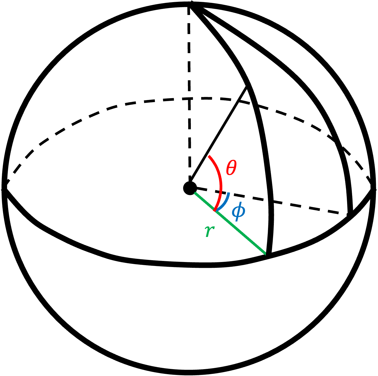
The Legendre polynomial arises from the spherical harmonics.

Fig. 13 Spherical Coordinate#
For Laplace equation on a spherical coordinate, it can be written.
Again, if we applied separation of variable to (127) and let \(\psi=R(r)\Theta(\theta)\Phi(\phi)\), we will have a set of ODEs and they are related to each others through eigenvalues \(\lambda\) and \(m\).
Here we take the zonal average (average over \(\phi\)), the second equation becomes 0 and the third equation can be written as,
From the equation above, we know the weighting function is \(\cos\theta\). Since \(d\sin\theta=\frac{1}{\cos\theta}d\theta\), we can further rewrite the above equation into
Then subtract \(\cos^2\theta\) from both terms and let \(\sin\theta=x\), we will have
which satisfies the Sturm-Liouville form given that the solution is bounded at both poles.
Following the typical procedure of solving Sturm-Liouville problem, assume the solution has a form of
which gives us
Substitute (132) and (133) into,
Examine each order, we have
we obtain
One can find, as long as we determine \(a_0\) and \(a_1\), we determine all of the higher order terms. i.e.,
We can find something interesting from the second and third lines of (137). The entire equation is truncated when \(\lambda = n(n-1)\). If we further set one of \(a_0\) or \(a_1\) equals 0, all of the even/odd terms vanish. This will form so-called Legendre Polynomials where,
x             = range(-1, 1, length=1000)
sum_Legendre_even = zeros(Complex, 7, 1000)
sum_Legendre_even[1,:] .= 1
count2        = 1
for n_max in 2:2:10  #give an even number
    a_even        = 1
    λ             = (n_max)*(n_max+1)
    Legendre_even = zeros(Complex, 100, 1000)
    Legendre_even[1,:] .= a_even
    count         = 2
    for n in 0:2:100
        a_even                 = ((n)*(n+1)-λ)/((n+1)*(n+2))*a_even
        Legendre_even[count,:] = a_even*x.^(float(n+2))
        count                  = count+1
    end
    sum_Legendre_even[count2+1,:] = sum(Legendre_even,dims=1)
    count2=count2+1
end

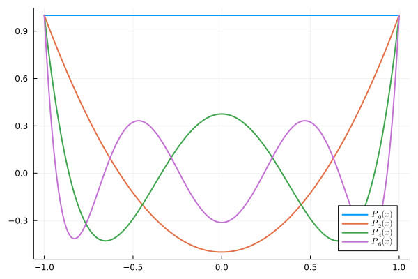
Fig. 14 An visualization of Legendre Polynomials with \(n=0,2,4,6\)#
From the figure above, one can find Legendre polynomials have maximum amplitude at both poles. This feature is caused by uneven weighting function in meridional direction. Recall that \(dx=d\sin\theta\), this indicates the grid spacing is much smaller at the poles (or the area is weighted by \(\cos\theta\)). When the “heat” around the equator is diffused to the pole, the energy will be more concentrated due to the Earth geometry. This geometry effect plays an important in Polar Amplification, where we usually see more significant rising temperature at the pole than the equator (and of course there are many other physical processes lead to this result, but the geometry is the 0th order influence). Similar things happen in tropical cyclone intensification, where the inflow of angular momentum can accelerate the tropical cyclone tangential wind. This effect is more significant around the inner core of tropical cyclone.
Generating Function and Recurrence Relations#
Like Bessel function, Legendre Polynomial also has a generating function. Let
For a given x, \(L(x,t)\) is a function which can be expanded in a power series about \(t=0\). When this is done, the coefficient of \(t^n\) is \(P_n(x)\), i.e.,
We can get some feeling for this result by looking at a few terms of the Maclaurin series (Taylor expansion at \(t=0\)). we know
for \(-1<w<1\). Put \(w=2xt-t^2\) to obtain
Expand the each of these powers and collect the coefficient of each power of \(t\) to obtain
The generating function is sometimes useful in deriving general results. For example, we can use the generating function to show that \(P_n(-1)=(-1)^n\). I will leave this questions to readers (HW).
Similar to Bessel function, there are also a few recurrence relations in Legendre Polynomials
This can be proved by an inductive argument (hint: differentiate the generating function with respect to \(t\) and multiply both sides with \(\sqrt(1-2xt+t^2)\). Then reorganize the equation). I will also let readers to complete the proof.
