Week 12: Wave Equation

Week 12: Wave Equation#

Problem Setup and Initial Conditions#

Waves are ubiquitous and especially central to atmospheric sciences. Vibration on any material with restoring forces can generate waves. The existence of restoring force implies the existence of 2nd-order derivatives in time. One of the most well-known wave equation is Hooke’s Law

(176)#

\begin{array}{r} \frac{d^{2} x}{d t^{2}} = - k x \end{array}

where the restoring force is equivalent to how much the material is stretched except with an opposite sign. This suggesting the force is always going against to the stretched direction. It’s not hard to find the solutions share a form of

(177)#

\begin{array}{r} x = a_{n} \cos (\sqrt{k} t) + b_{n} \sin (\sqrt{k} t) \end{array}

The coefficients in (175) will be determined by the given initial values of $x$ and $x_{t}$ . This is the general setup of wave solutions, where only the temporal structure is considered.

Wave Solution with Space and Time Structures#

Here we will consider a slightly more complicated case where the propagating over a space (i.e., we are observing wave at both space and time.). Therefore, the original equation can be rewritten as

(178)#

\begin{array}{r} y_{t t} = c^{2} y_{x x}; for 0 < x < L, t > 0 \end{array}

with initial and boundary conditions

(179)#

\begin{array}{r} \begin{aligned} y (x, 0) & = f (x),; y_{t} (x, 0) = g (x) \\ y (0, t) & = y (L, t) = 0 \end{aligned} \end{array}

Using separation of variable, one can expect that the solution shares a form of (leave this practice to readers)

(180)#

\begin{array}{r} y_{n} (t) = X_{n} (x) T_{n} (t) = [a_{n} \cos (\frac{n π c t}{L}) + b_{n} \sin (\frac{n π c t}{L})] \sin (\frac{n π x}{L}) \end{array}

In most cases, we can satisfy the initial condition with finite sum of $a_{n}$ and $b_{n}$ . We therefore attempt a solutions

(181)#

\begin{array}{r} \begin{aligned} y (x, t) & = \sum_{n = 1}^{\infty} y_{n} (x, t) \\ = \sum_{n = 1}^{\infty} [a_{n} \cos (\frac{n π c t}{L}) + b_{n} \sin (\frac{n π c t}{L})] \sin (\frac{n π x}{L}) \end{aligned} \end{array}

using initial condition, we know

(182)#

\begin{aligned} y (x, 0) & = \sum_{n = 1}^{\infty} a_{n} \sin (\frac{n π x}{L}) = f (x) \end{aligned}

indicating

(183)#

\begin{array}{r} \begin{aligned} a_{n} & = \frac{2}{L} \int_{0}^{L} f (ξ) \sin (\frac{n π ξ}{L}) d ξ \\ \frac{n π c}{L} b_{n} & = \frac{2}{L} \int_{0}^{L} g (ξ) \sin (\frac{n π ξ}{L}) d ξ \end{aligned} \end{array}

Example 1

Suppose a string with fixed ends at $x = 0$ and $x = π$ , with initial conditions of

\begin{array}{r} f (x) = {\begin{cases} x for 0 \leq x \leq \frac{π}{2} \\ π - x for \frac{π}{2} < x \leq π \end{cases} \end{array}

and

g (x) = x (1 - \cos (x))

We also assume $c = 1$ , which represents the propagating speed of waves

From (181), we know the solution has a form of

\begin{array}{r} y (x, t) = \sum_{n = 1}^{\infty} [a_{n} \cos (n t) + b_{n} \sin (n t)] \sin (n x) \end{array}

where

\begin{array}{r} a_{n} = \frac{2}{π} \int_{0}^{π} f (ξ) \sin (\frac{n π ξ}{L}) d ξ = \frac{4 \sin (\frac{n π}{2})}{n^{2} π} \end{array}

and

\begin{array}{r} \begin{aligned} b_{n} & = \frac{2}{n π c} \int_{0}^{π} g (ξ) \sin (\frac{n π ξ}{L}) d ξ \\ = \frac{- 2}{n^{2}} (- 1)^{n} + \frac{2 (- 1)^{n}}{n^{2} - 1} \\ = \frac{2}{n^{2} (n^{2} - 1)} (- 1)^{n} \end{aligned} \end{array}

Now considering a more complicated case, where we have external forcing. i.e.,

(184)#

\begin{array}{r} \begin{aligned} y_{t t} & = c^{2} y_{x x} + x; for 0 < x < L, t > 0 \\ y (0, t) & = y (L, t) = 0, \\ y (x, 0) & = x (L - x) = f (x) \\ y_{t} (x, 0) & = x (1 + \cos (\frac{π x}{L})) = g (x) \end{aligned} \end{array}

Similar to how we deal with heat equation with external forcing, we can assume the solution shares a form of

(185)#

y (x, t) = Y (x, t) + ψ (x)

Substitute (185) back to (184), we can have a homogeneous equation for $Y (x, t)$ .

(186)#

Y_{t t} = c^{2} Y_{x x}

and an 2nd-order ODE for the forcing term i.e.,

(187)#

c^{2} ψ^{^{″}} = - x

Integrating (187) twice, we have

(188)#

ψ (x) = - \frac{x^{3}}{6 c^{2}} + α x + β

Now, look at boundary conditions,

(189)#

y (0, t) = 0 = Y (0, t) + ψ (0) = Y (0, t) + β

To make (189) a homogeneous problem, we choose $b e t a = 0$ . For the other boundary condition,

(190)#

y (L, t) = 0 = Y (L, t) + ψ (L) = Y (L, t) - \frac{L^{3}}{6 c^{2}} + α L

Let

(191)#

α = \frac{L^{2}}{6 c^{2}}

we can have the same homogeneous equation at the second boundary.

(191) indicates that

(192)#

ψ = - \frac{x^{3}}{6 c^{2}} + \frac{L^{2}}{6 c^{2}} x = \frac{x}{6 c^{2}} (L^{2} - x^{2})

With the result above, we can rewrite the entire set of wave equation to

(193)#

\begin{array}{r} \begin{aligned} Y_{t t} & = c^{2} Y_{x x}; for 0 < x < L, t > 0 \\ Y (0, t) & = Y (L, t) = 0, \\ Y (x, 0) & = x (L - x) - ψ = x (L - x) - \frac{x}{6 c^{2}} (L^{2} - x^{2}) \\ Y_{t} (x, 0) & = x (1 + \cos (\frac{π x}{L})) = g (x) \end{aligned} \end{array}

We know how to solve this problem.

Wave Motion in an Unbounded Medium#

Consider the problem

(194)#

\begin{array}{r} \begin{aligned} y_{t t} & = c^{2} y_{x x}; for \infty < x < \infty, t > 0 \\ y (x, 0) & = f (x) \\ y_{t} (x, 0) & = 0 \end{aligned} \end{array}

Similarly, using separation of variable, we have

(195)#

\begin{array}{r} \begin{aligned} X^{^{″}} + λ X & = 0 \\ T^{^{″}} + λ c^{2} T & = 0 \end{aligned} \end{array}

The first equation has a solution of

(196)#

\begin{array}{r} X = \sum_{n = 0}^{\infty} a_{n} \cos (k x) + b_{n} \sin (k x) \end{array}

where

(197)#

\begin{array}{r} k = \frac{n π}{L} \end{array}

Here we make the increment between two adjacent wave numbers small ( $\sim 0$ ). i.e.,

(198)#

\begin{array}{r} d k = \frac{π}{L} \sim 0; where L \to \infty \end{array}

We can rewrite (196) into

(199)#

\begin{array}{r} X = \frac{1}{π} \sum_{n = 0}^{\infty} A_{n} \cos (k x) + B_{n} \sin (k x) d k = \frac{1}{π} \int_{k = 0}^{\infty} A_{k} \cos (k x) + B_{k} \sin (k x) d k \end{array}

and

(200)#

\begin{array}{r} T_{k} = \cos (k c t) \end{array}

(readers can think about why T has a constant multiple of Fourier consine function as its solution?)

According to (199), we know

(201)#

\begin{array}{r} \begin{aligned} A_{n} & = \int_{- \infty}^{\infty} f (ξ) \cos (k ξ) d ξ \\ B_{n} & = \int_{- \infty}^{\infty} f (ξ) \sin (k ξ) d ξ \end{aligned} \end{array}

and the completed equation is

(202)#

\begin{array}{r} y (x, t) = \frac{1}{π} \int_{k = 0}^{\infty} [a_{k} \cos (k x) + b_{k} \sin (k x)] \cos (k c t) d k \end{array}

Example 2

Solve the problem on a real line with initial displacement of $f (x)$ and 0 initial velocity

y (x, 0) = f (x) = e^{- | x |}

All we have to do is calculate the Fourier integral for $A_{n}$ and $B_{n}$ . These are

A_{n} = \int_{- \infty}^{\infty} e^{- | ξ |} \cos (k ξ) d ξ = \frac{2}{π (1 + k^{2})}

and

B_{n} = 0

because $e^{- | x | \sin (k x)}$ is an odd function.

The solution is

y (x, t) = \frac{2}{π} \int_{0}^{\infty} \frac{1}{1 + k^{2}} \cos (k x) \cos (k c t) d k

D’Alembert’s Solutions, Characteristic Lines, and Dispersion Relationship#

Jean Le D’Alembert (1717-1783) developed a simple method to approach the wave equations, known as the D’Alembert’s Wave Solutions. In optical physics and atmospheric wave dynamics, it has a special name dispersion relationships. i.e., the relation between wave length and wave speed.

Specifically, the D’Alembert’s wave solution describes

(203)#

y (x, t) = F (ξ) + G (η) = \frac{1}{2} [f (x - c t) + f (x + c t)] + \frac{1}{2 c} \int_{x - c t}^{x + c t} g (x^{'}) d x^{'}

where

(204)#

\begin{array}{r} \begin{aligned} ξ & = x - c t \\ η & = x + c t \end{aligned} \end{array}

To show that, we first observe (195) and we can find the following two characteristic equations

(205)#

\begin{array}{r} \begin{aligned} (\frac{\partial}{\partial t} - c \frac{\partial}{\partial x}) y & = 0 \\ (\frac{\partial}{\partial t} + c \frac{\partial}{\partial x}) y & = 0 \end{aligned} \end{array}

while (205) is a slightly more complicated form, we can try to convert it into a simpler question

(206)#

\begin{array}{r} \begin{aligned} \frac{\partial}{\partial ξ} y & = 0 \\ \frac{\partial}{\partial η} y & = 0 \end{aligned} \end{array}

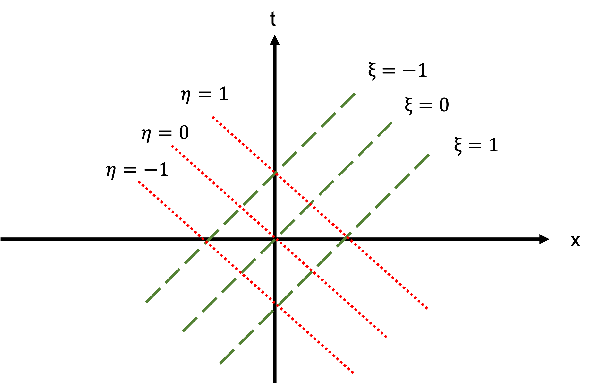
(206) is an ODE for $y$ , which can be solved with direct integration. One can easily find y is independent of $ξ$ and $η$ . That means we gonna apply certain linear transform from $x, t$ plane to $ξ, η$ plane where $y$ is a constant along $ξ$ and $η$ .

To find the corresponding Jacobian matrix, we can first observe the original equation. (205) can be written as

(207)#

\begin{array}{r} \begin{aligned} < (- c, 1) | (y_{x}, y_{t}) > & = 0 \\ < (c, 1) | (y_{x}, y_{t}) > & = 0 \end{aligned} \end{array}

$y_{x}$ and $y_{t}$ represent how $y$ changes with respect to $x$ and $t$ . If we assign the first coordinate as $x$ and the second coordinate as $t$ , the first equation above indicates that $y$ is constant along the direction of $(- c, 1)$ or $y$ is conserved along each line of $x = - c t + η$ . As long as $η$ is given, we know the solution of $y$ . This also implies that $y$ is a function of $η$ . The same idea can be applied to $ξ$ .

../_images/DAlambert.png — Fig. 16 The D’Alambert’s wave solution.#

Combining both, we have

(208)#

\begin{array}{r} u (x, t) = F (ξ) + G (η) \end{array}

Here we demonstrate how to derive the D’Alambert’s wave solution. According to the initial condition of the wave position, we know

(209)#

\begin{array}{r} \begin{aligned} y (x, 0) & = F (ξ) + G (η) = f (x) \\ y_{t} (x, 0) & = \frac{\partial F (ξ)}{\partial ξ} \frac{\partial ξ}{\partial t} + \frac{\partial G (η)}{\partial η} \frac{\partial η}{\partial t} = - c F^{^{'}} (ξ) + c G^{^{'}} (η) = g (x) \end{aligned} \end{array}

Here if we properly choose an integral for the second equation (I will show that in a seconds), we will have

(210)#

\begin{array}{r} \begin{aligned} y (x, 0) & = F (x) + G (x) = f (x) \\ \int_{x_{0}}^{x} g (w) d w & = - c F (x) + c G (x) \end{aligned} \end{array}

Then we can represent $y$ with the linear combination of the two equations above.

(211)#

\begin{array}{r} \begin{aligned} F (x - c t) & = \frac{1}{2} f (x - c t) - \frac{1}{2 c} \int_{x_{0}}^{x - c t} g (w) d w \\ G (x + c t) & = \frac{1}{2} f (x + c t) + \frac{1}{2 c} \int_{x_{0}}^{x + c t} g (w) d w \end{aligned} \end{array}

Adding both together, we have solutions

(212)#

\begin{array}{r} u (x, t) = F (x - c t) + G (x + c t) = \frac{1}{2} [f (x - c t) + f (x + c t)] + \frac{1}{2 c} \int_{x - c t}^{x + c t} g (w) d w \end{array}

Week 12: Wave Equation

Contents

Week 12: Wave Equation#

Problem Setup and Initial Conditions#

Wave Solution with Space and Time Structures#

Wave Motion in an Unbounded Medium#

D’Alembert’s Solutions, Characteristic Lines, and Dispersion Relationship#